previous  index  next 

28. Dielectrics II: Response to External Fields; Boundary Conditions

    Michael Fowler, UVa

Introduction: Constitutive Relation

Experimentally, it is very well established that nonconducting solids respond to an applied electric field by becoming to some degree polarized, which on a macroscopic level is the same as generating a dipole density. Obviously, this phenomenon is relevant in many areas of science and engineering$—$consequently, there are a lot of names describing the same thing.

In the following, we assume that the response (the polarization $\overrightarrow{P}$) of the dielectric medium to the applied electric field $\overrightarrow{E}$ is linear, a very good approximation in practice for the field strengths normally encountered. For now, we’ll also assume the response is isotropic, there are important exceptions (single crystal materials) we’ll return to later.

The electric susceptibility ${\chi }_e$ is defined by

$\overrightarrow{P}={\epsilon }_0{\chi }_e\overrightarrow{E},$

so ${\chi }_e$ is dimensionless.  It measures, obviously, how susceptible the medium is to being polarized by an electric field.  (The subscript e is for electric, as opposed to magnetic, susceptibility.  We’ll get to the magnetic response later.)

But we could have asked: how does the displacement $\overrightarrow{D}$ respond to the external field?

(Wait, isn’t that really the same question?  $\overrightarrow{D}={\epsilon }_0\overrightarrow{E}+\overrightarrow{P},$ right?  Yes, but bear with me.)

This is called the constitutive relation

$\overrightarrow{D}=\epsilon \overrightarrow{E},\epsilon ={\epsilon }_0\left(1+{\chi }_e\right)$

and $\epsilon$ is the electric permittivity.  So ${\epsilon }_0$ is the vacuum permittivity.

There’s still more notation!

The dimensionless dielectric constant $\kappa$ is defined as the ratio of the permittivity to the vacuum permittivity:

$$\kappa =\frac{\epsilon }{{\epsilon }_0}=1+{\chi }_e.$$

$\kappa$ is also called the relative permittivity.

If the permittivity has no spatial variation, then

$$\overrightarrow{\nabla }\cdot \overrightarrow{E}=\frac{\overrightarrow{\nabla }\cdot \overrightarrow{D}}{\epsilon }=\frac{{\rho }_{\text{free}}\left(\overrightarrow{r}\right)}{\epsilon },$$

note the free charge density.

That is to say, in a uniform medium, the fields, and therefore potentials, produced by a given charge distribution are the same as in a vacuum, but scaled down by a factor $\epsilon /{\epsilon }_0.$  

We’ll find that $\epsilon >{\epsilon }_0$ always, the charge within the molecules moves to partially shield external charge.  Hence for a given charge a capacitor with a dielectric medium rather than nothing between the plates will have that much less potential difference between them$—$meaning its capacitance is increased by a factor $\epsilon /{\epsilon }_0,$ of great practical importance.

Boundary Conditions

Recall from the previous lecture that

$\overrightarrow{D}\left(\overrightarrow{r}\right)=-\overrightarrow{\nabla }{\displaystyle \int d^3{r}^{\prime }\frac{{\rho }_{\text{free}}\left({\overrightarrow{r}}^{\prime }\right)}{4\pi \left|\overrightarrow{r}-{\overrightarrow{r}}^{\prime }\right|}}+\overrightarrow{\nabla }\times {\displaystyle \int d^3{r}^{\prime }}\frac{{\overrightarrow{\nabla }}^{\prime }\times \overrightarrow{P}\left({\overrightarrow{r}}^{\prime }\right)}{4\pi \left|\overrightarrow{r}-{\overrightarrow{r}}^{\prime }\right|},$

so in the absence of free charge, $\overrightarrow{\nabla }\cdot \overrightarrow{D}=0.$ Therefore, for a thin pillbox disc at the interface, Gauss’ theorem gives

$\left({\overrightarrow{D}}_2-{\overrightarrow{D}}_1\right)\cdot \widehat{\overrightarrow{n}}=0.$ 

The right-hand side will be nonzero if there really is free charge ${\sigma }_{\text{free}}$ qt the interface, which there usually isn’t. 

The normal component of the electric field $\overrightarrow{E}$ is discontinuous at the interface, from the excess local (bound) charge inherent in the polarization discontinuity. 

The other boundary condition is established by using Stokes’ theorem for integrating around a loop contour half in the dielectric, half out, as shown.

Since $\overrightarrow{\nabla }\times \overrightarrow{E}=0,$ the surface integral vanishes, and the line integral gives

$\left({\overrightarrow{E}}_2-{\overrightarrow{E}}_1\right)\times \overrightarrow{n}=0.$

In other words, the component of the electric field parallel to the surface, ${\overrightarrow{E}}_{\parallel },$ is continuous across the surface.

Dielectric Boundary Value Problems

Image Method for Point Charge

First, we examine the standard problem of a point charge in a semi-infinite $\left(z>0\right)$ dielectric having permittivity ${\epsilon }_1,$ the charge being distance $d$ from the plane interface with a second dielectric, permittivity ${\epsilon }_2,$ filling the other half of space $\left(z<0\right)$. 

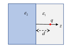
The point charge is the only unbound charge in the system, there will of course be unbalanced bound charge on the interface since the permittivity changes there.  (In the special case ${\epsilon }_2=\infty$, the “bound charge” is no longer bound$—$this is our old problem of a charge above a grounded conducting plane.  But for finite ${\epsilon }_2,$ the field penetrates the boundary.)  

The equations are

$\begin{array}{l}\overrightarrow{\nabla }\cdot \overrightarrow{D}={\epsilon }_1\overrightarrow{\nabla }\cdot \overrightarrow{E}=\rho z>0\\ \overrightarrow{\nabla }\cdot \overrightarrow{D}={\epsilon }_2\overrightarrow{\nabla }\cdot \overrightarrow{E}=0z<0\\ \underset{z\to 0^{-}}{\lim {\epsilon }_2{E}_z}=\underset{z\to 0^{+}}{\lim {\epsilon }_1{E}_z}\end{array}$

Of course $\overrightarrow{\nabla }\times \overrightarrow{E}=0$  so $\overrightarrow{E}=-\overrightarrow{\nabla }\phi$  for some potential, and $E_x,E_y$ are continuous at the border, $E_z$ has a step discontinuity from the sheet of unbalanced bound charge.

This problem is a lot like the charge above a conducting plane, except that this time we need to find the electric field on the other side too.  It turns out that there is a simple image solution.

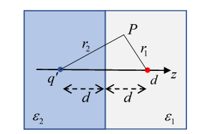
For $z>0$, we take there to be an image charge $q^{\prime }$ at the point $-d$.  Then

$$\phi \left(z>0\right)=\frac{1}{4\pi {\epsilon }_1}\left(\frac{q}{r_1}+\frac{q^{\prime }}{r_2}\right)$$

and for $z<0$ we assume (admittedly with hindsight)

$$\phi \left(z<0\right)=\frac{1}{4\pi {\epsilon }_2}\frac{q^{″}}{r_1},$$

since there is no real charge for $z<0.$  Notice this means that in the region where the charge isn’t, the lines of electric field are straight, and radiating from the charge (which itself is in the other half).

Labeling the radial coordinate in the $z=0$ plane as $\rho ,$ at $z=0$ we can see that

$\frac{\partial }{\partial z}\left(\frac{1}{r_1}\right)=-\frac{\partial }{\partial z}\left(\frac{1}{r_2}\right),\frac{\partial }{\partial \rho }\left(\frac{1}{r_1}\right)=\frac{\partial }{\partial \rho }\left(\frac{1}{r_2}\right).$ It follows that the boundary conditions are satisfied by the charge and the images $q^{\prime },q^{″}$ in the appropriate regions provided (matching the normal components of $\overrightarrow{D}$ )

$q-q^{\prime }=q^{″},$ 

and from the continuity of the tangential components of $\overrightarrow{E}$ 

$\frac{q+q^{\prime }}{{\epsilon }_1}=\frac{q^{″}}{{\epsilon }_2}.$

Solving for the image charges,

$\begin{array}{l}{q}^{\prime }=-\left(\frac{{\epsilon }_2-{\epsilon }_1}{{\epsilon }_2+{\epsilon }_1}\right)q,\\ q^{″}=\left(\frac{2{\epsilon }_2}{{\epsilon }_2+{\epsilon }_1}\right)q.\end{array}$ 

Exercise:  Plot the field lines in the two regions. Draw two plots, for ${\epsilon }_2>{\epsilon }_1$ and ${\epsilon }_2<{\epsilon }_1.$

Finding the (bound) surface charge density at the interface is straightforward: it’s equal to $-\overrightarrow{\nabla }\cdot \overrightarrow{P}$, and $\overrightarrow{P}={\epsilon }_0\chi \overrightarrow{E}.$ The jump in susceptibility $\chi$ generates a delta function in charge density $—$a surface layer,

$\sigma =P_{1z}-P_{2z}=\left({\epsilon }_1-{\epsilon }_0\right)E_{z1}-\left({\epsilon }_2-{\epsilon }_0\right)E_{z2}$ and putting in the values from the image solution,

$\begin{array}{c} E_{1z}=-\frac{\partial {\phi }_1}{\partial z}=-\frac{q}{4\pi {\epsilon }_1}{\nabla }_z\left(\frac{1}{r_1}\right)-\frac{q^{\prime }}{4\pi {\epsilon }_1}{\nabla }_z\left(\frac{1}{r_2}\right)\\ =-\frac{q-q^{\prime }}{4\pi {\epsilon }_1}\frac{d}{{\left({\rho }^2+d^2\right)}^{3/2}}=-\frac{q}{2\pi }\frac{{\epsilon }_2}{{\epsilon }_1}\frac{1}{{\epsilon }_2+{\epsilon }_1}\cdot \frac{d}{{\left({\rho }^2+d^2\right)}^{3/2}}\end{array}$

$\begin{array}{c}{E}_{2z}=-\frac{\partial \phi }{\partial z}=-\frac{q^{″}}{4\pi {\epsilon }_2}{\nabla }_z\left(\frac{1}{r_1}\right)\\ =-\frac{q^{″}}{4\pi {\epsilon }_2}\frac{d}{{\left({\rho }^2+d^2\right)}^{3/2}}=-\frac{q}{2\pi }\frac{1}{{\epsilon }_2+{\epsilon }_1}\cdot \frac{d}{{\left({\rho }^2+d^2\right)}^{3/2}}\end{array}$

giving

$\sigma =-\frac{q}{2\pi }\cdot \frac{{\epsilon }_0}{{\epsilon }_1}\cdot \frac{{\epsilon }_2-{\epsilon }_1}{{\epsilon }_2+{\epsilon }_1}\cdot \frac{d}{{\left({\rho }^2+d^2\right)}^{3/2}}$

Exercise: Does this charge density agree qualitatively with the field lines you plotted? Look at both cases.

Dielectric Sphere in Uniform Field

This is basically a weaker version of the conducting sphere in a uniform field: the sphere becomes uniformly polarized, the discontinuity of $\overrightarrow{P}$at the spherical surface is equivalent to a charge layer that generates a uniform field inside the sphere, partially cancelling the applied field; and a dipole field outside.

These assertions are proved by taking the external applied field to have potential ${\phi }_{\text{ext}}\left(\overrightarrow{r}\right)=-E_{0}r\cos \theta ,$ and noting that the boundary conditions of continuous electric field parallel to the surface and continuous electric displacement $\overrightarrow{D}=\epsilon \overrightarrow{E}$ perpendicular to the surface, that is,

$\begin{array}{c}{\left.\frac{\partial {\phi }_{\text{in}}}{\partial \theta }\right|}_{r=a}={\left.\frac{\partial {\phi }_{\text{out}}}{\partial \theta }\right|}_{r=a}\\ {\left.\epsilon \frac{\partial {\phi }_{\text{in}}}{\partial r}\right|}_{r=a}={\left.{\epsilon }_0\frac{\partial {\phi }_{\text{out}}}{\partial r}\right|}_{r=a}\end{array}$

can be satisfied by taking potentials having the angular symmetry of the imposed field, meaning $P_1\left(\theta \right)$:

${\phi }_{\text{in}}\left(\overrightarrow{r}\right)=Ar\cos \theta ,{\phi }_{\text{out}}\left(\overrightarrow{r}\right)=-E_{0}r\cos \theta +\frac{C}{r^2}\cos \theta .$

The boundary conditions give:

$Aa=-E_{0}a+\frac{C}{a^2},\epsilon A=-{\epsilon }_0{E}_0-\frac{2{\epsilon }_{0}C}{a^3}.$

These equations are easily solved to find

$A=-\left(\frac{3{\epsilon }_0}{2{\epsilon }_0+\epsilon }\right)E_0,C=\left(\frac{\epsilon -{\epsilon }_0}{\epsilon +2{\epsilon }_0}\right)a^3{E}_0.$

Notice that there is no need to bother with higher order $P_l$'s: we have only two equations to satisfy, so we get two adjustable parameters by having a uniform field inside and a dipole field outside,and once we have satisfied the boundary conditions (and our results make physical sense: nondivergent fields at the origin and at infinity), the uniqueness theorem assures us that we’ve solved the problem. Besides, the material is spherically symmetric, the imposed field has $P_1$ symmetry, the problem is linear, there is no mechanism for manufacturing, say, a quadrupole moment.

Now the $Ar\cos \theta =-\left(\frac{3{\epsilon }_0}{2{\epsilon }_0+\epsilon }\right)E_{0}r\cos \theta$ term is the total electric potential inside.

It is equal to the applied field potential $-E_{0}r\cos \theta$ plus a field generated by the polarization, so that field must be $\left(\frac{{\epsilon }_0-\epsilon }{2{\epsilon }_0+\epsilon }\right)E_{0}r\cos \theta .$

For another way of seeing the same thing, recall we showed earlier that a dielectric sphere with uniform polarization $\overrightarrow{P}$generates its own internal electric field ${\overrightarrow{E}}_P=-\overrightarrow{P}/3{\epsilon }_0,$ so this must be the difference between the actual field and the applied external field,

$\left(\frac{3{\epsilon }_0}{2{\epsilon }_0+\epsilon }\right)E_0-E_0=\left(\frac{{\epsilon }_0-\epsilon }{2{\epsilon }_0+\epsilon }\right)E_0=-\frac{P}{3{\epsilon }_0}.$

So the polarization is proportional to the actual electric field inside the sphere (of course)

$P=-3{\epsilon }_0\left(\frac{{\epsilon }_0-\epsilon }{2{\epsilon }_0+\epsilon }\right)E_0=-\left({\epsilon }_0-\epsilon \right)E_{\text{inside}}.$

This is just $D={\epsilon }_{0}E+P$ inside the material.

Exercises

1. Sketch the effective charge density from the polarization, and sketch the field lines.

2. Put a thick spherical shell of uniform dielectric, inner radius $a$ and outer radius $b,$ in a constant electric field, find the potential everywhere. Sketch the effective surface charge densities from the polarization, and sketch the field lines.

Spherical Cavity in Uniform Dielectric with Outside Uniform Field Applied

The first point to clarify is what is this applied field? Suppose we take a slab of dielectric with a small spherical cavity, and put it in a uniform electric field, say between two oppositely charged plates.The field inside the dielectric is reduced from that between the plates in vacuum, because there is polarization charge on the flat surfaces of the dielectric. Hence in this problem the "outside field" is the field inside the dielectric, from charged plates + the polarization charge density on the flat surfaces.

The mathematics is identical to that for the dielectric sphere in an external field, except that the $\epsilon$’s are reversed. The field in the cavity is uniform, stronger than the outside field since $\epsilon >{\epsilon }_0,$ and given by ${\overrightarrow{E}}_{\text{in}}=\left[3\epsilon /\left(2\epsilon +{\epsilon }_0\right)\right]{\overrightarrow{E}}_0.$ The additional outside field is that of a dipole $\overrightarrow{p}=4\pi {\epsilon }_0\left[\left(\epsilon -{\epsilon }_0\right)/\left(2\epsilon +{\epsilon }_0\right)\right]a^3{\overrightarrow{E}}_0.$ 

Exercise: plot the field lines. Be careful! Sketch the dipole field, and see where it strengthens, and where it opposes, the external field.Your field lines must be closer together where the field is stronger.

previous  index  next