54  Waveguides I

    Michael Fowler, UVa

Introduction

As detailed in the previous lecture, the idea of confining a propagating electromagnetic wave in a metal tube was first proposed by J. J. Thomson in 1893, and mathematically analyzed by Lord Rayleigh in 1897.  Rayleigh discovered that waves below a certain cutoff frequency would not propagate. 

The first attempt at actually constructing waveguides for possible commercial use was by George Southworth at Bell Labs in the 1930's. Unaware of Rayleigh's work, the group there was at first bewildered by their lack of success in transmitting low-frequency waves.  Fortunately, a mathematician colleague who had escaped from Russia in 1917 recreated Rayleigh’s analysis, and the experimenters raised the frequency to one that would propagate (the first message transmitted was “send money”.)

Here is Southworth demonstrating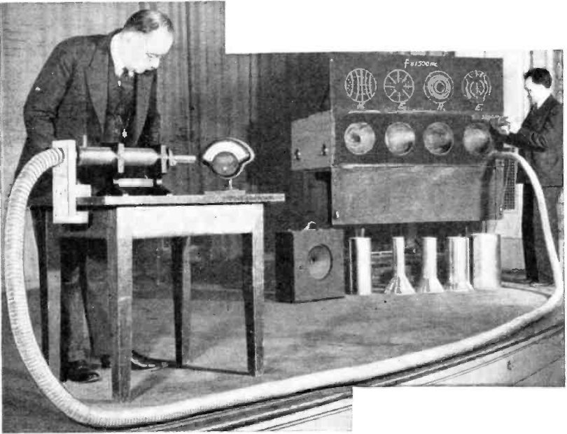

an early waveguide in 1938. (Notice the field diagrams above the transmitter.)

The development of radar in the Second World War led to a rapid development of waveguide technology.  Waveguides were used to feed the power from the oscillator (a magnetron, invented at the University of Birmingham) to the antenna. This work was done at the MIT Rad Lab, a team led by Purcell, and including Schwinger, Bethe and others.

Nowadays, waveguides are mainly used for high frequency power transmission (typically in the gigahertz range) in radar, of course, (see picture)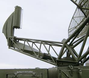 but also in accelerators.  The waveguide transverse dimensions are comparable to the wavelength being transmitted.  For some accelerator installations, this is roughly the same as a 2"x4" wooden beam.  The similarity proved useful on one occasion: a granting agency checking progress of accelerator construction was bamboozled by "waveguides" that were in fact two by fours painted with copper paint (this from an anonymous source).

Waveguides are also used in microwave transmitters: these were the original underwater long lines, carrying most of the telephone traffic, now largely replaced by fiber optics. 

In preparing this lecture, I used Feynman’s Lectures in Physics, Volume 2, Chapter 24. I highly recommend that as an introduction. I also used Griffiths, Introduction to Electrodynamics, Third Edition, Section 9.5, which gives more detail than Feynman on TE, TM; ω, k relationships, etc. Of course, much of the lecture follows Jackson.

Preliminaries: Boundary Conditions

First: for a Perfect Conductor

In thinking about electromagnetic waves being guided, in other words directed down some kind of tube, the first thing to establish is how does the tube constrain the wave, in other words, what are the boundary conditions?

The second practical question is: how quickly are the currents induced in the boundary conducting material draining energy from the wave?

We'll begin by considering the wall to be a perfect conductor: there can be no electric field inside this conductor, it would instantly be shielded out by the charges adjusting on the surface, so the electric field inside the guide, on approaching the wall, is normal to the wall surface, and terminates at a layer of surface charge.  (Any electric field at the surface parallel to the surface would create a large current in the conductor.) 

What about the magnetic field? There can be a static magnetic field inside a conductor, a magnet will work through a copper sheet.  But you can't have an oscillating field inside a perfect conductor, since it necessarily has an accompanying electric field.  There can’t be a normal component to the magnetic field, that would require a monopole layer, but there can be a parallel component terminated by a layer of surface current.

Second: A Real Conductor: Skin Depth

(Note: this section is a reminder of material already covered in lectures 37 and 47.)

Notation: We will use $z$ in this section for depth into the conducting material, the notation Jackson himself used in the earlier treatment of skin depth (p 220), where the same equations were derived.  (Doubtless he uses $\xi$ here since he now wants to reserve $z$ for distance along the wave guide, but I want to make very clear that we’ve already done this problem.)

For a real conductor, like copper, the idealized delta function layers of charge and current on the “perfect conductor” obviously spread to some finite (if small) depth, so the electric field to some extent penetrates the conductor, generating currents and consequently heat, and therefore attenuating the wave.

The depth of penetration is called the skin depth, labeled $\delta ,$ the currents generated are eddy currents.

The displacement current (the $\partial \overrightarrow{E}/\partial t$ term) is negligible compared to the free electron current in a good conductor, so the appropriate equations are (including Ohm’s law, and $\mu ,\sigma$ refer to values for the conductor)

$\overrightarrow{\nabla }\times \overrightarrow{H}=\overrightarrow{j}=\sigma \overrightarrow{E},\overrightarrow{\nabla }\times \overrightarrow{E}=-\mu \frac{\partial \overrightarrow{H}}{\partial t},$ 

so for fields having time dependence $e^{-i\omega t},$ 

${\nabla }^2\overrightarrow{H}=-i\mu \sigma \omega \overrightarrow{H}.$ 

We take the surface to be the $\left(x,y\right)$ plane, and so measure depth into the conductor as $z$ (the equations then coincide with those in lecture 47, on impedance of a metal reflector).

Taking the field outside the conductor to be $\overrightarrow{H}=\left(H_x,0,0\right)$ then inside the conductor, $z\ge 0,$

$H_x\left(z,t\right)=h\left(z\right)e^{-i\omega t},$ 

and $h\left(z\right)$ satisfies

$\left(\frac{d^2}{d{z}^2}+i\mu \sigma \omega \right)h\left(z\right)=0,$ 

assuming field variation in the $z$-direction is far more rapid than in other directions, so we can take ${\nabla }^2=d^2/d{z}^2.$ 

A solution $e^{ikz}$ works provided $k^2=i\mu \sigma \omega ,$ or $k=\pm \left(1+i\right)\sqrt{\frac{\mu \sigma \omega }{2}}.$ 

The solution has to be the sign giving exponential decay of the field into the conductor, that gives a decay length, the skin depth:

$\delta =\sqrt{\frac{2}{\mu \sigma \omega }}.$ 

In terms of $\delta ,$ the magnetic field inside the conductor is

$H_x\left(z\right)=H_x{e}^{-\left(1-i\right)z/\delta },$ 

neglecting here the possible slow variations parallel to the surface.

Now $\overrightarrow{\nabla }\times \overrightarrow{H}=\overrightarrow{j}=\sigma \overrightarrow{E},$ from which the electric field inside the conductor

$\overrightarrow{E}=\left(1/\sigma \right)\left(1-i\right)\left(1/\delta \right)\left(\overrightarrow{n}\times \overrightarrow{H}\right)e^{-\left(1-i\right)z/\delta }=\sqrt{\mu \omega /2\sigma }\left(1-i\right)\left(\overrightarrow{n}\times \overrightarrow{H}\right)e^{-\left(1-i\right)z/\delta }.$ 

This can also be written in terms of the impedance, as in lecture 47.  In this regime, the impedance $Z=\sqrt{\mu /\epsilon }\approx \sqrt{\mu \omega /i\sigma },$ and this internal electric field is $E_y\left(z\right)=Z{H}_x\left(z\right).$

This field is generated purely by the oscillating magnetic field, and is much smaller than the electric field outside the conductor in general.   But, unlike the outside electric field, this internal field is tangential to the surface, and therefore there is also a nonzero tangential electric field infinitesimally above the surface, in the tube, and so a nonzero Poynting vector, an energy flow, into the surface from the wave:

$-\frac{1}{2}\mathrm{Re}\left[\overrightarrow{n}\cdot \overrightarrow{E}\times {\overrightarrow{H}}^{\ast }\right]=\frac{1}{4}\mu \omega \delta {\left|H_x\right|}^2=\frac{1}{4}\sqrt{\frac{2\mu \omega }{\sigma }}{\left|H_x\right|}^2=\frac{1}{2\sqrt{2}}\left|Z\right|{\left|H_x\right|}^2.$

From Ohm's law inside the conductor $\overrightarrow{J}=\sigma \overrightarrow{E}=\left(1/\delta \right)\left(1-i\right)\left(\overrightarrow{n}\times \overrightarrow{H}\right)e^{-\left(1-i\right)z/\delta }$, it's straightforward to show this energy all goes into Joule heating. 

Notice that for a given field strength, power loss goes up with frequency as $\sqrt{\omega }.$   It also goes as $1/\sqrt{\sigma },$ because it goes as $\sigma E^2,$ but $E\sim H/\sqrt{\sigma },$ and the volume of dissipation per unit area is given by the penetration depth $\sim 1/\sqrt{\sigma }.$ 

Summary: Fields Near the Surface

The key is that the surface can have charge density and current density, spread through a depth of order $\delta .$ 

There can be a strong perpendicular electric field outside the surface, from the layer of charge.  Such a field inside would dissipate quickly, moving charge to or from the surface layer. As discussed above, there is a small tangential electric field, continuous across the surface.

There can be a strong tangential magnetic field outside the surface, generated by surface currents. As we have seen, tangential fields inside the conductor attenuate at the decay length.

Any outside perpendicular magnetic field would continue into the conductor (there are no sheets of magnetic charge!), and decay rapidly from eddy currents (this is of course an oscillating field) so any such field must be very weak.

Waveguides

Notation: from now on, $z$ measures distance along the waveguide.

The first waveguide was Heaviside’s coaxial cable, discussed in the previous lecture.

Coaxial Cable

Commercial electrical power is AC, with a frequency of 50 or 60 Hz, depending on country, it is transmitted by wires, and therefore radiates power. But the loss of power by radiation is trivial compared with the ohmic heating loss.  However, AC radiation goes as the fourth power of frequency (we’ll be discussing this a little later in the course), so going up from 50Hz to megahertz makes all the difference. The most common solution to transmitting high frequency signals is the coaxial cable,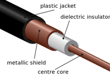 two concentric cylindrical surfaces, with equal and opposite currents and charges at any point on the cable, so no external fields, and hence no radiation. (Image from Wikipedia.) This is hooked up to some oscillator generating the field, so evidently waves go down the cable.

Hollow Cylindrical Waveguide

(Jackson 8.2.  Note: cylindrical just means the cross section is always the same, not necessarily circular.)

Deriving Transverse Differential Equations for E_z, B_z

The coaxial cable and the two-wire model discussed in the previous lecture are easy to visualize in terms of local capacitance and inductance.  But in fact, as J. J. Thomson suggested and Lord Rayleigh analyzed, we can send waves down a single hollow conductor: it's straightforward to write down Maxwell's equations and solve them.

We take it that the oscillating source generates waves with a time dependence $e^{-i\omega t}.$ 

Inside the waveguide, Maxwell’s equations are

$\begin{array}{l}\overrightarrow{\nabla }\times \overrightarrow{E}=i\omega \overrightarrow{B}\overrightarrow{\nabla }\cdot \overrightarrow{B}=0\\ \overrightarrow{\nabla }\times \overrightarrow{B}=-i\mu \epsilon \omega \overrightarrow{E}\overrightarrow{\nabla }\cdot \overrightarrow{E}=0\end{array}$ .

It follows that

$\begin{array}{l}\left({\nabla }^2+\mu \epsilon {\omega }^2\right)\overrightarrow{E}=0,\\ \left({\nabla }^2+\mu \epsilon {\omega }^2\right)\overrightarrow{B}=0.\end{array}$ 

We’ll now assume that all components of $\overrightarrow{E}$ vary in the $z$ direction, down the guide, as $e^{ikz},$  so

$\left(\frac{{\partial }^2}{\partial x^2}+\frac{{\partial }^2}{\partial y^2}-k^2+\mu \epsilon {\omega }^2\right)\overrightarrow{E}\left(x,y\right)=0.$ 

Evidently we’re now looking at a 2-D ${\nabla }^2$ problem: Jackson writes

$\left({\partial }^2/\partial x^2+{\partial }^2/\partial y^2\right)={\nabla }_t{}^2,$

 $t$ for transverse, meaning in the plane perpendicular to the direction of the wave guide.

The approach is to write out Maxwell’s equations in terms of transverse and parallel (to $z$ ) components, then write the transverse $\overrightarrow{E}$ and $\overrightarrow{B}$ fields just in terms of $E_z,B_z$ as follows (I decided to follow Griffiths’ presentation, which is a bit more transparent than Jackson’s here. I'll connect with Jackson's approach in the next lecture.):

$\begin{array}{l}\overrightarrow{\nabla }\times \overrightarrow{E}=\dot{\overrightarrow{B}}=i\omega \overrightarrow{B}:\overrightarrow{\nabla }\times \overrightarrow{B}={\mu }_0{\epsilon }_0\dot{\overrightarrow{E}}=-\frac{i\omega }{c^2}\overrightarrow{E}\\ \frac{\partial E_y}{\partial x}-\frac{\partial E_x}{\partial y}=i\omega B_z\frac{\partial B_y}{\partial x}-\frac{\partial B_x}{\partial y}=-\frac{i\omega }{c^2}{E}_z\\ \frac{\partial E_z}{\partial y}-ik{E}_y=i\omega B_x\frac{\partial B_z}{\partial y}-ik{B}_y=-\frac{i\omega }{c^2}{E}_x\\ ik{E}_x-\frac{\partial E_z}{\partial x}=i\omega B_{y}ik{B}_x-\frac{\partial B_z}{\partial x}=-\frac{i\omega }{c^2}{E}_y.\end{array}$ 

Note now that we can choose two equations for $E_x:$   

$\begin{array}{c}-\frac{i\omega }{c^2}{E}_x=\frac{\partial B_z}{\partial y}-ik{B}_y,\\ ik{E}_x=\frac{\partial E_z}{\partial x}+i\omega B_y.\end{array}$ 

The strategy is to get $E_x,E_y,B_x,B_y$ all in terms of only $E_z,B_z.$ 

So, we need to eliminate $B_y$ between the two equations above, multiplying the first by $\omega ,$ the second by $k$ and adding:

$\begin{array}{l}\frac{-i{\omega }^2}{c^2}{E}_x+i{k}^2{E}_x=\omega \frac{\partial B_z}{\partial y}+k\frac{\partial E_z}{\partial x},\\ E_x=\frac{i}{{\left(\omega /c\right)}^2-k^2}\left(\omega \frac{\partial B_z}{\partial y}+k\frac{\partial E_z}{\partial x}\right).\end{array}$ 

Similarly,

$\begin{array}{l}{E}_y=\frac{i}{{\left(\omega /c\right)}^2-k^2}\left(k\frac{\partial E_z}{\partial y}-\omega \frac{\partial B_z}{\partial x}\right),\\ B_x=\frac{i}{{\left(\omega /c\right)}^2-k^2}\left(k\frac{\partial B_z}{\partial x}-\frac{\omega }{c^2}\frac{\partial E_z}{\partial y}\right),\\ B_y=\frac{i}{{\left(\omega /c\right)}^2-k^2}\left(k\frac{\partial B_z}{\partial y}+\frac{\omega }{c^2}\frac{\partial E_z}{\partial x}\right).\end{array}$ 

We have already shown that

$\left[\frac{{\partial }^2}{\partial x^2}+\frac{{\partial }^2}{\partial y^2}+{\left(\frac{\omega }{c}\right)}^2-k^2\right]E_z=0.$ 

and similarly

$\left[\frac{{\partial }^2}{\partial x^2}+\frac{{\partial }^2}{\partial y^2}+{\left(\frac{\omega }{c}\right)}^2-k^2\right]B_z=0.$ 

So, we have 2-D  ${\nabla }^2$ equations for $E_z,B_z$ and from the earlier equations, it’s straightforward to compute $E_x,E_y,B_x,B_y$ from $E_z,B_z.$ So in principle we’ve solved the problem.

Electric and Magnetic Boundary Conditions

Of course, to actually find solutions of the differential equations for $E_z,B_z$, we need the boundary conditions!

Let’s start with $E_z$:  this is easy, we need $E_z=0$ at the boundary, since the metal is taken to be a perfect conductor (and even if it isn't, the skin depth must be far smaller than the waveguide size, or it wouldn't work).

$B_z$ is more tricky, we know that $B_{\perp }=0$ at the surface, but $B_z$ isn’t in general zero.  However, we can use $\overrightarrow{\nabla }\times \overrightarrow{B}={\mu }_0{\epsilon }_0\left(\partial \overrightarrow{E}/\partial t\right)$ and look near the surface in the direction tangential to the surface but also perpendicular to $z$ $—$call it $y$, so $x$ is normal to the surface (see figure). 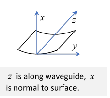 Thus, the $y$ component of $\overrightarrow{\nabla }\times \overrightarrow{B}={\mu }_0{\epsilon }_0\dot{\overrightarrow{E}}$ is

${\left(\overrightarrow{\nabla }\times \overrightarrow{B}\right)}_y=\frac{\partial B_z}{\partial n}-\frac{\partial B_n}{\partial z}={\mu }_0{\epsilon }_0\frac{\partial E_y}{\partial t}.$ 

In this equation, we already know that close enough to the perfectly conducting (in our approximation) surface, the tangential $E_y$ and the normal $B_n=B_x$ are both identically zero, so we conclude that the boundary condition we need is:

$\partial B_z/\partial n=0.$ 

Boundary Conditions for Field z-Components

We now see that $E_z\left(x,y\right),B_z\left(x,y\right)$ satisfy exactly the same differential equation but with different boundary conditions:    

$E_z=0,\frac{\partial B_z}{\partial n}=0.$

The differential equation is a 2D eigenvalue equation for $E_z$ (or for $B_z$ ):

$\left[\frac{{\partial }^2}{\partial x^2}+\frac{{\partial }^2}{\partial y^2}\right]E_z\left(\text{or }{B}_z\right)=\left(k^2-{\left(\frac{\omega }{c}\right)}^2\right)E_z\left(\text{or }{B}_z\right),$ 

and different boundary conditions will give in general different allowed eigenvalues (think standing waves in an organ pipe with both ends open or one end closed, one open). 

Therefore, in general, for consistency, at least one of $E_z,B_z$ must be zero. This leads to three classes of modes.

Actually there are exceptional (termed hybrid) modes in some geometries with $z$ -direction electric and magnetic fields, the most important being for rectangular cross-section waveguides. See the full discussion in the next lecture.

Possible Modes: TM, TE, TEM

The possibilities are:

TM  (transverse magnetic) solutions: zero longitudinal (parallel to the cable) magnetic field.

That is, $B_z=0$  everywhere.

( Of course $E_z=0$ at the surface, as always.)

Now $E_x=\frac{i}{{\left(\omega /c\right)}^2-k^2}\left(\omega \frac{\partial B_z}{\partial y}+k\frac{\partial E_z}{\partial x}\right)$  and $E_y=\frac{i}{{\left(\omega /c\right)}^2-k^2}\left(k\frac{\partial E_z}{\partial y}-\omega \frac{\partial B_z}{\partial x}\right).$

Therefore for $B_z\equiv 0,$ the transverse electric field

${\overrightarrow{E}}_t=\frac{ik}{{\left(\omega /c\right)}^2-k^2}{\overrightarrow{\nabla }}_t{E}_z,$

and correspondingly

${\overrightarrow{B}}_t=\left(\omega /k\right)\widehat{\overrightarrow{z}}\times {\overrightarrow{E}}_t.$ 

TE  (transverse electric) solutions: $E_z=0$ everywhere, $\partial B_z/\partial n=0$ at surface.

From $B_x=\frac{i}{{\left(\omega /c\right)}^2-k^2}\left(k\frac{\partial B_z}{\partial x}-\frac{\omega }{c^2}\frac{\partial E_z}{\partial y}\right)$ and $B_y=\frac{i}{{\left(\omega /c\right)}^2-k^2}\left(k\frac{\partial B_z}{\partial y}+\frac{\omega }{c^2}\frac{\partial E_z}{\partial x}\right),$

 we find for $E_z\equiv 0$  that

${\overrightarrow{B}}_t=\frac{ik}{{\left(\omega /c\right)}^2-k^2}{\overrightarrow{\nabla }}_t{B}_z,$

and

${\overrightarrow{E}}_t=-\left(\omega /c\right)\widehat{\overrightarrow{z}}\times {\overrightarrow{B}}_t.$ 

TEM:  $B_z=E_z=0$ everywhere. As mentioned above in discussing the coaxial cable, this is equivalent to a 2-D electrostatics problem, the boundary cross-section needs a minimum of two separate components, at different potentials in the 2-D problem.

Solving for the Modes

In the next lecture, we’ll find these modes in detail for the solvable (and important) case of a rectangular cross section pipe, and also analyze the analogous modes in a rectangular cavity.

previous  index  next