55  Waveguides II

    Michael Fowler, UVa

Introduction

In the previous lecture, we established that there were three different possible modes for traveling waves in a hollow cylindrical (not in general circular) conducting waveguide, following (more or less) the presentation in Griffiths. Here we’ll investigate further, more closely following Jackson.

Notation:  

1.  We repeat the equations from the previous lecture, but now with dielectric filling, so replacing $1/c^2$ with $\mu \epsilon .$

2.  For the given frequency $\omega ,$ we label the free space wave number

$$k_0=\omega \sqrt{\mu \epsilon }.$$

TM  (transverse magnetic) solutions: zero longitudinal (parallel to the guide) magnetic field.

That is, $B_z=0$ everywhere in the waveguide, $E_z=0$ at the conducting surface (as always).

We found for TM waves, the longitudinal electric field $E_z$ satisfies $\left[\frac{{\partial }^2}{\partial x^2}+\frac{{\partial }^2}{\partial y^2}+\mu \epsilon {\omega }^2-k^2\right]E_z=0,$ 

and  the transverse $\left(t\right)$ electric field ${\overrightarrow{E}}_t=\frac{ik}{\mu \epsilon {\omega }^2-k^2}{\overrightarrow{\nabla }}_t{E}_z,$ magnetic field ${\overrightarrow{B}}_t=\left(\mu \epsilon \omega /k\right)\widehat{\overrightarrow{z}}\times {\overrightarrow{E}}_t.$ 

TE  (transverse electric) solutions: $E_z\equiv 0$ everywhere in the waveguide, $\partial B_z/\partial n=0$ at the surface.

the longitudinal magnetic field $B_z$ satisfies $\left[\frac{{\partial }^2}{\partial x^2}+\frac{{\partial }^2}{\partial y^2}+\mu \epsilon {\omega }^2-k^2\right]B_z=0,$

and the transverse fields are ${\overrightarrow{B}}_t=\frac{ik}{\mu \epsilon {\omega }^2-k^2}{\overrightarrow{\nabla }}_t{B}_z,$ ${\overrightarrow{E}}_t=-\left(\omega /k\right)\widehat{\overrightarrow{z}}\times {\overrightarrow{B}}_t.$ 

TEM:  $B_z=E_z=0$ everywhere.

Wave Impedance

 From these equations, and using $\overrightarrow{B}=\mu \overrightarrow{H},$ the transverse magnetic and electric fields satisfy

${\overrightarrow{H}}_t=\frac{\pm 1}{Z}\widehat{\overrightarrow{z}}\times {\overrightarrow{E}}_t,$ 

(for $e^{\pm ikz}$ ) where $Z,$ the wave impedance, is given by (remember we’ve switched from $\overrightarrow{B}$ to $\overrightarrow{H}$ )

$Z=\frac{k}{\epsilon \omega }=\frac{k}{k_0}\sqrt{\frac{\mu }{\epsilon }}\text{(TM),}Z=\frac{\mu \omega }{k}=\frac{k_0}{k}\sqrt{\frac{\mu }{\epsilon }}\text{(TE),}{k}_0=\omega \sqrt{\mu \epsilon }.$ 

Recall that (lecture 46) $\sqrt{\mu /\epsilon }$ is the impedance for a free space plane wave. (See the zigzag picture given below for some insight into the other term.)

The impedance is important when waveguides are put together, or waveguides are connected to sources or sinks: the impedances need to match, otherwise there will be reflection of the wave and consequent inefficiency.

The units are ohms, typical coax cable is around 75 ohms for TV signals.

Solving for the Modes: TEM

Let's first look for TEM modes. Recall now our earlier discussion of the coaxial cable: that was clearly a TEM mode. To get more quantitative, since $B_z\equiv 0,$ for a TEM mode, the now (only two-dimensional!) electric field satisfies $\overrightarrow{\nabla }\times {\overrightarrow{E}}_{TEM}=0$ so we can write

${\overrightarrow{E}}_{TEM}={\overrightarrow{\nabla }}_t\phi e^{-i\left(\omega t-kz\right)}$ 

with the two-dimensional potential satisfying

${\nabla }_t{}^2\phi =0.$ 

For the usual coaxial cable, we’d take polar coordinates. In fact, this is a familiar electrostatics problem, we know the surfaces are perfect conductors, the solution for the coaxial case is a radial electric field, the potential goes as $A\ln \rho ,$ the field as $A/\rho .$ The magnetic field $B$ is in circles, of strength $\sqrt{\mu \epsilon }A/\rho ,$ and of course both have the factor $e^{-i\left(\omega t-kz\right)}.$

But what about TEM modes in just a hollow waveguide?  This same analysis shows that the transverse electric field is again like an electrostatic field, but this time with a potential constant over the whole boundary$—$the unique possible field is identically zero: so there cannot be a TEM mode in a single hollow conducting pipe!  Essentially, TEM modes need two surfaces, and the transverse electric field look like the electrostatic field from opposite charges on the two (conducting) surfaces. For example, for two parallel cylinders (or wires) see the diagrams in lecture 15.

Notation!  We’ll follow Jackson closely in this section, so we replace both $E_z\left(x,y,z\right)$ and $B_z\left(x,y,z\right)$ with $\psi \left(x,y\right)e^{-i\left(\omega t-kz\right)}.$

TM Modes

For TM waves, we have identically zero $B_z,$ and nonzero

$$E_z\left(x,y,z\right)=\psi \left(x,y\right)e^{-i\left(\omega t-kz\right)}$$

where

$\left[\frac{{\partial }^2}{\partial x^2}+\frac{{\partial }^2}{\partial y^2}\right]\psi \left(x,y\right)=\left(k^2-\mu \epsilon {\omega }^2\right)\psi \left(x,y\right),$ 

which we write as

$\left({\nabla }_t{}^2+{\gamma }^2\right)\psi =0$.

Here

$${\gamma }^2=\mu \epsilon {\omega }^2-k^2.$$

  ${\gamma }^2$ cannot be negative since we need wave-type solutions on the transverse plane, to satisfy $E_z=0$  at all boundaries:  negative ${\gamma }^2$ would give exponentials.  Given the boundary condition, the differential equation will have a set of eigenvalues  ${\gamma }_{\lambda }{}^2,\lambda =1,2,3\dots$ and for each one there will be waves having $z$-direction wavenumber

$k_{\lambda }{}^2=\mu \epsilon {\omega }^2-{\gamma }_{\lambda }{}^2.$ 

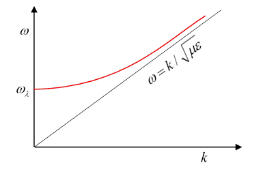
Notice this means there is a cutoff (minimum) frequency for each family,

${\omega }_{\lambda }=\frac{{\gamma }_{\lambda }}{\sqrt{\mu \epsilon }}.$

above which the $z$ -direction wavenumber will be 

$k_{\lambda }=\sqrt{\mu \epsilon }\sqrt{{\omega }^2-{\omega }_{\lambda }{}^2}.$

At high frequencies, $\omega \cong k/\sqrt{\mu \epsilon },$ the waves move close to the speed of light in the dielectric.

Near the threshold $\omega \cong {\omega }_{\lambda }$ the group velocity

$v_g=d\omega /dk=\sqrt{\mu \epsilon }\sqrt{1-\frac{{\omega }_{\lambda }^2}{{\omega }^2}}$ 

 is very slow, going to zero.  (On the other hand, the phase velocity, $v_p=\omega /k$, goes to infinity at threshold.  From $\mu \epsilon \omega d\omega =kdk,$ note that $v_g{v}_p=1/\mu \epsilon .$ )

*Optional Aside: The Zigzag Picture for a Rectangular Pipe

To reduce clutter, we’ll just take vacuum in this section.

We just mention this picture (first suggested in 1903) as a slightly different way of imagining the wave going down the guide.

The fields have ordinary traveling wave behavior $e^{ikz}$ along the tube, but standing wave behavior in the perpendicular directions, to satisfy the boundary conditions.

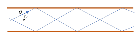
For a particular mode, a way to visualize this is to imagine a wave aimed into the tube at an angle so that it bounces up and down in a zigzag path, reflected in turn by the top and bottom of a rectangular waveguide, and it will bounce off the sides too, we won’t try to draw that, the math is straightforward, as you’ll see.   We could also add in a wave aimed in at the same angle downwards, as shown here. (The relative phase of the two waves determines if the mode is TE or TM.)

The wave will interfere with itself destructively unless the parallel segments of the wave are in phase with each other. This means the angle $\theta$ can only have certain values, as discussed below.

These bouncing waves are ordinary light waves, with $\overrightarrow{E},\overrightarrow{B}$ perpendicular to each other and to ${\overrightarrow{k}}^{\prime }$ as usual.

Taking ${\overrightarrow{k}}^{\prime }$ to be at an angle $\theta$ to the $z$ direction, the $k$ in $e^{ikz}$ is given by $k=k^{\prime }\cos \theta .$  For the lowest mode, we need the wavelengths in the perpendicular directions to be twice the tube dimensions, that is, ${\overrightarrow{k}}^{\prime }\cdot \widehat{\overrightarrow{x}}=\pi /a,{\overrightarrow{k}}^{\prime }\cdot \widehat{\overrightarrow{y}}=\pi /b,$ to give simple standing waves in the perpendicular directions, eliminating destructive interference.

Now the zigzagging wave is just light in a vacuum (we’re assuming no dielectric in the waveguide), so $\omega =c{k}^{\prime },$ and ${k^{\prime }}^2=k^2+{\left(\pi /a\right)}^2+{\left(\pi /b\right)}^2,$ so generalizing in the obvious way to all standing waves in the perpendicular directions,

$\omega =c\sqrt{k^2+{\left(m\pi /a\right)}^2+{\left(n\pi /b\right)}^2},$ 

for positive integers $m,n.$   

Rectangular Waveguide: Details

For TE waves, there is no electric field pointing down the pipe, but a nonzero $H_z$,

and, now following Jackson, we write $H_z=\psi \left(x,y\right)e^{-i\left(\omega t-kz\right)},$ with

$\left[\frac{{\partial }^2}{\partial x^2}+\frac{{\partial }^2}{\partial y^2}+{\gamma }^2\right]\psi \left(x,y\right)=0,{\gamma }^2=\mu \epsilon {\omega }^2-k^2,$

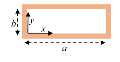
 and boundary conditions:

$\frac{\partial \psi }{\partial n}=0\text{ at }x=0,a\text{ and at }y=0,b.$

The solutions are (check these$—$note the origin is at bottom left in the diagram)

${\psi }_{mn}\left(x,y\right)=H_0\cos \left(\frac{m\pi x}{a}\right)\cos \left(\frac{n\pi y}{b}\right),{\gamma }_{mn}^2={\pi }^2\left(\frac{m^2}{a^2}+\frac{n^2}{b^2}\right).$ 

Then from ${\gamma }^2=\mu \epsilon {\omega }^2-k^2,$ we have

$\omega =\frac{1}{\sqrt{\mu \epsilon }}\sqrt{k^2+{\left(\frac{m\pi }{a}\right)}^2+{\left(\frac{n\pi }{b}\right)}^2},$

For $a>b,$ the lowest frequency mode is $m=1,n=0$ 

${\omega }_{1,0}=\frac{\pi }{a\sqrt{\mu \epsilon }}$ 

 and the TE_1,0 fields are (from Jackson):

$\begin{array}{l}{H}_z=H_0\cos \left(\frac{\pi x}{a}\right)e^{i\left(kz-\omega t\right)},\\ H_x=-\frac{ika}{\pi }{H}_0\sin \left(\frac{\pi x}{a}\right)e^{i\left(kz-\omega t\right)},\\ E_y=i\frac{\omega a\mu }{\pi }{H}_0\sin \left(\frac{\pi x}{a}\right)e^{i\left(kz-\omega t\right)}.\end{array}$ 

Exercise:  Check that these follow from ${\overrightarrow{B}}_t=\frac{ik}{\mu \epsilon {\omega }^2-k^2}{\overrightarrow{\nabla }}_t{B}_z,$ ${\overrightarrow{E}}_t=-\left(\omega /k\right)\widehat{\overrightarrow{z}}\times {\overrightarrow{B}}_t.$

For a given frequency $\omega$ of wave sent down the pipe, the $z$-direction wave number will be

$k_{1,0}=\sqrt{\mu \epsilon }\sqrt{{\omega }^2-{\omega }_{1,0}^2}.$ 

$\omega {}_{1,0}$ is the cutoff frequency: if the incoming $\omega <{\omega }_{1,0},$ the wave number is imaginary, meaning the wave exponentially decays in the pipe.  (What about the Poynting vector?) 

Exercise:  try sketching the fields in one wavelength for this 1,0 mode, taking $\omega >\omega {}_{1,0}$.   This is in fact the mode most widely used commercially: for $a>b,$ there is no TM mode until the smaller of twice cutoff or $\left(a/b\right)$ times cutoff, so no mixing problems.  For the rectangular pipe, as we are about to show, in general there are TE and TM modes at the same frequency.

For the TM modes, $E_z\left(x,y\right)$ has to go to zero at the walls, so $E_z\left(x,y\right)=E_0\sin \left(\frac{m\pi x}{a}\right)\sin \left(\frac{n\pi y}{b}\right)$, and the lowest mode will be 1,1, a higher cutoff frequency than the lowest TE mode, but for a general TM mode $\left(m,n\right)$ the value of ${\gamma }_{mn}^2={\pi }^2\left(\frac{m^2}{a^2}+\frac{n^2}{b^2}\right)$ and hence the frequency is the same as for the corresponding TE. (This is in contrast to, for example, a waveguide with a circular cross-section, or indeed almost any cross-section other than rectangular.)

Exercise:  Examine carefully this representation of field lines for two modes in a rectangular waveguide, and answer the following:

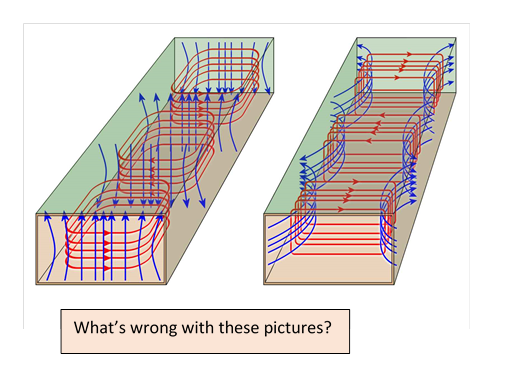
(a) Identify the modes allegedly represented.

(b) There are some definite errors here!  Re-sketch the diagrams correctly.

(c) Sketch the charge density and current density in the walls for this field configuration.

I found this online years ago, but it has been taken down. I suspect the authors are not anxious to have their work attributed.

Energy loss and Attenuation

For real walls, as opposed to perfect conductors, the wave penetrated $\sim \delta$ into the walls, where Joule heating takes place, and energy is drained from the wave. We've found the formula for loss per unit area of wall surface in terms of the parallel magnetic field at the wall. We also know how to find the power being delivered down the guide by the wave. The rate of power loss is proportional to the square of the field, as is the power delivered, so the power going down the guide will decrease exponentially, in Jackson's notation

$P\left(z\right)=P_0{e}^{-2{\beta }_{\lambda }z}$ 

so the attenuation coefficient (for mode $\lambda$ )  is

${\beta }_{\lambda }=-\frac{1}{2P}\frac{dP}{dz}$ 

where the power drain is found by integrating around the circumference to find the loss rate per unit length of pipe:

$-\frac{dP}{dz}=\frac{1}{2\sigma \delta }{\displaystyle \underset{C}{\oint }{H}_{\parallel }^{2}d\ell .}$ 

This is straightforward given the waveguide shape and the mode. Consult Jackson for details of the calculation. He ends with an estimate, we'll just look at it and interpret the terms. The attenuation coefficient is

${\beta }_{\lambda }=\sqrt{\frac{\epsilon }{\mu }}\frac{1}{\sigma {\delta }_{\lambda }}\left(\frac{C}{2A}\right)\frac{\sqrt{\omega /{\omega }_{\lambda }}}{\sqrt{1-{\left({\omega }_{\lambda }/\omega \right)}^2}}\left[{\xi }_{\lambda }+{\eta }_{\lambda }{\left({\omega }_{\lambda }/\omega \right)}^2\right].$ 

For ordinary waveguide shapes, it turns out that $\xi ,\eta$ are numbers of order unity, and $\eta =0$ for TM (it comes from the component of magnetic field in the $z$ -direction for TE waves).  The $C/A$ term encodes the relative surface area to volume, the "geometric factor".  The crucial physics is that at high frequencies the $\sqrt{\omega /{\omega }_{\lambda }}$ is the dominating factor, it comes directly from the Joule heating, so energy loss increases with frequency in this regime.  But it also increases going to low frequencies (meaning just above cutoff) :  the $1/\sqrt{1-{\left({\omega }_{\lambda }/\omega \right)}^2}$ blows up$—$that’s the group velocity going to zero, so little power is being delivered down the pipe, but the Joule heating is still happening.  Evidently the attenuation has a minimum value somewhere.

For TM modes $\left(\eta \equiv 0\right),$ the attenuation has a simple frequency dependence, and the minimum loss rate is at $\omega =\sqrt{3}{\omega }_{\lambda }.$

Exercise:  Check the last statement.

 (Jackson 8.6: Perturbation of Boundary Conditions:  we'll skip this).

previous  index  next