previous  index  next 

67.  The Lienard-Weichert Potentials and Fields

    Michael Fowler, UVa

Potentials from a Moving Point Charge

The correct expressions for the potentials of a moving point charge $\phi$ and $\overrightarrow{A}$ were found long ago (before relativity!) by Lienard and Wiechert. They are:

$$\phi \left(\overrightarrow{x},t\right)=\frac{1}{4\pi {\epsilon }_0}{\left[\frac{q}{R\left(1-\overrightarrow{\beta }\cdot \overrightarrow{n}\right)}\right]}_{\text{ret}},\overrightarrow{A}=\frac{{\mu }_{0}c}{4\pi }{\left[\frac{q\overrightarrow{\beta }}{R\left(1-\overrightarrow{\beta }\cdot \overrightarrow{n}\right)}\right]}_{\text{ret}}.$$The bracket ${\left[\right]}_{\text{ret}}$ means that the contents must be evaluated at the retarded time, meaning the potential is determined by the position (and velocity) of the charge at time earlier by $t_{\text{ret}}$ such that $c{t}_{\text{ret}}=R,$ the distance of the charge at that instant from the point of observation.  In other words, information about the charge position encoded in the potential is transmitted at the speed of light.

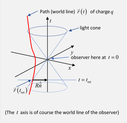
In this diagram, we take the origin to be at the point and time of the observation, to simplify the picture.  The field observed at $\overrightarrow{r}=0,t=0$ arises from the point in spacetime where the world path of the charge intersected the backward light cone from the point of observation.

This naturally gives rise to the expressions above, except for that extra factor $1-\overrightarrow{\beta }\cdot \widehat{\overrightarrow{n}}$.  Where did that come from?

It arises because we must integrate over all past times, using a delta function to pick out the right one:

$$\phi \left(\overrightarrow{x},t\right)=\frac{1}{4\pi {\epsilon }_0}{\displaystyle \underset{t^{\prime }<t}{\int }\frac{q}{R}\delta \left(t^{\prime }-R\left(t^{\prime }\right)/c\right)d{t}^{\prime }}.$$  From the well-known formula

$${\displaystyle \int g\left(t\right)\delta \left(f\left(t\right)\right)}dt=g\left(t_0\right)/\left|f^{\prime }\left(t_0\right)\right|$$  (assuming a single zero of $f\left(t\right)$ at $t_0$ ), we find

$$\phi \left(\overrightarrow{x},t\right)=\frac{1}{4\pi {\epsilon }_0}\frac{q}{R_{\text{ret}}}\frac{1}{\left(1-{\overrightarrow{\beta }}_{\text{ret}}\cdot \widehat{\overrightarrow{n}}\right)},$$because the term multiplying $\dot{R}\left(t_{\text{ret}}\right)$ that comes from differentiating the delta function is just the component of the velocity in the direction $\widehat{\overrightarrow{n}}$ from the charge at $\overrightarrow{r}\left(t_{\text{ret}}\right)$ to the point $\overrightarrow{x}=0$ at which we are measuring the field.

This is rather a formal derivation: is there some more intuitive way to see where the factor comes from?  Try this.  As we discussed long ago in talking about Green's functions, the charge is a source, from which the field emanates.  Imagine it to be constantly transmitting little packets of information, proportional to its strength. We detect the field at some other point from the rate at which these packets arrive. If we're moving towards the source, they come in that much faster, by exactly this term.  This is just the same as the Doppler effect. (This argument is not invoking time dilation, relativity, etc.:  Lienard and Wiechert wrote it long before Einstein!)

Electric and Magnetic Fields

Having found the potentials, all we need do to evaluate the fields is to differentiate:

$$\overrightarrow{B}=\overrightarrow{\nabla }\times \overrightarrow{A},\overrightarrow{E}=-\overrightarrow{\nabla }\phi -\partial \overrightarrow{A}/\partial t$$But this isn’t so easy $—$ $\overrightarrow{\nabla }\times \overrightarrow{A}$ means differentiating $\overrightarrow{A}$ with respect to $\overrightarrow{x}$ at fixed $t.$ Now the values of $\overrightarrow{A}$ at two neighboring points $\overrightarrow{x}$ and $\overrightarrow{x}+\Delta \overrightarrow{x}$ at time $t$ correspond to different times $t_{\text{ret}}$.  This will affect $R\widehat{\overrightarrow{n}}$ and must be included in differentiating the potentials.

Let’s start by considering $R$, the distance from $\overrightarrow{r}\left(t_{\text{ret}}\right)$ to $\overrightarrow{x}.$  We take it that the path the particle follows, $\overrightarrow{r}\left(t_{\text{ret}}\right)$, has been set in advance. This means that $R$ can be thought of as a function of $\overrightarrow{x}$ and $t_{\text{ret}}$ only, its dependence on $t_{\text{ret}}$ being given by the known function $\overrightarrow{r}\left(t_{\text{ret}}\right)$.   The velocity of the particle at time $t_{\text{ret}}$ is obviously $\partial \overrightarrow{r}\left(t_{\text{ret}}\right)/\partial t_{\text{ret}}$.   (Since $t_{\text{ret}}$ is defined as a function of $t$ from $R=\left|\overrightarrow{x}-\overrightarrow{r}\left(t_{\text{ret}}\right)\right|=c\left(t-t_{\text{ret}}\right)$, this may seem confusing.  Why isn’t the velocity just $\partial \overrightarrow{r}\left(t_{\text{ret}}\right)/\partial t$?  The point is that $\overrightarrow{r}\left(t_{\text{ret}}\right)$ is the position at the earlier time $t_{\text{ret}}$, and if the particle is moving at constant velocity $\overrightarrow{v}$, for example, then when one second of the “earlier time” has elapsed, the particle will have moved $\overrightarrow{v}$ meters. For such a particle, the path is $\overrightarrow{r}\left(t_{\text{ret}}\right)=\overrightarrow{v}{t}_{\text{ret}}$. Think of a car going along a road at 60 mph, passing milestones each of which has a clock.  As it passes each clock, the clock will read exactly one minute later than the previous clock did as the car passed. Now imagine someone observing this journey with a telescope from far away. That observer will also see the milestone clocks each reading one minute later as the car passes$—$and each such observation is of a retarded position at the corresponding retarded time.)

For fixed $\overrightarrow{x},$ 

$$\partial R/\partial t_{\text{ret}}=-\widehat{\overrightarrow{n}}\cdot \overrightarrow{v}$$because $R\widehat{\overrightarrow{n}}$ points from $\overrightarrow{r}\left(t_{\text{ret}}\right)$ to $\overrightarrow{x}$, so if $\overrightarrow{r}\left(t_{\text{ret}}\right)$ is moving at $\overrightarrow{v}$, $R\widehat{\overrightarrow{n}}$ is being eaten up from the back at the rate given by the right-hand side of the above equation, that is, the component of $\overrightarrow{r}\left(t_{\text{ret}}\right)$ ’s velocity along the line of the vector.

Now from $R=c\left(t-t_{\text{ret}}\right),$ differentiating $R$ with respect to time at fixed $\overrightarrow{x},$ 

$$\frac{\partial R}{\partial t}=c\left(1-\frac{\partial t_{\text{ret}}}{\partial t}\right)=\frac{\partial R}{\partial t_{\text{ret}}}\frac{\partial t_{\text{ret}}}{\partial t}=-\widehat{\overrightarrow{n}}\cdot \overrightarrow{v}\frac{\partial t_{\text{ret}}}{\partial t}$$from this we find

$$\frac{\partial t_{\text{ret}}}{\partial t}=\frac{1}{1-\widehat{\overrightarrow{n}}\cdot \overrightarrow{\beta }},\overrightarrow{\beta }=\overrightarrow{v}/c.$$Or

$$\frac{\partial }{\partial t}=\left(1-\widehat{\overrightarrow{n}}\cdot \overrightarrow{\beta }\right)\frac{\partial }{\partial t_{\text{ret}}}$$both partial derivatives being understood to be at fixed $\overrightarrow{x}$.

(Actually this is easy to see. Consider the one-dimensional case: $\overrightarrow{r}\left(t_{\text{ret}}\right)$ is moving along the x-axis towards $\overrightarrow{x}$ (which is itself on the axis) at steady speed $v$.  If $\Delta t_{\text{ret}}$ is one second, what is Δt? If at $t_{\text{ret}}=0$ the distance from $\overrightarrow{r}\left(t_{\text{ret}}\right)$ to $\overrightarrow{x}$ is $R,$ then $t=R/c.$ When $t_{\text{ret}}=1$ second, $\overrightarrow{r}\left(t_{\text{ret}}\right)$ has moved $v$ meters towards $\overrightarrow{x}$, and the corresponding $t$ is now $t=1+\left(R-v\right)/c.$ Hence $\Delta t_{\text{ret}}/\Delta t=1/\left(1-v/c\right).$ )

Now for the grad operator. The grad operator takes derivatives at constant $t$ by definition, so since $R=c\left(t-t_{\text{ret}}\right),$

$$\overrightarrow{\nabla }R=-c\overrightarrow{\nabla }{t}_{\text{ret}}.$$But we can also approach $\overrightarrow{\nabla }R$ from $R=\left|\overrightarrow{x}-\overrightarrow{r}\left(t_{\text{ret}}\right)\right|$.  We must first differentiate with respect to $\overrightarrow{x}$ at constant $t_{\text{ret}},$ then add the contribution from the variation of $\overrightarrow{r}\left(t_{\text{ret}}\right)$, but that latter is just the contribution from varying $t_{\text{ret}}$ at fixed $\overrightarrow{x}.$  

Thus

$$\overrightarrow{\nabla }R={\overrightarrow{\nabla }}_{\overrightarrow{x}}R+\frac{\partial R}{\partial t_{\text{ret}}}\overrightarrow{\nabla }{t}_{\text{ret}}=\widehat{\overrightarrow{n}}-\left(\widehat{\overrightarrow{n}}\cdot \overrightarrow{v}\right)\overrightarrow{\nabla }{t}_{\text{ret}}.$$Putting this together with $\overrightarrow{\nabla }R=-c\overrightarrow{\nabla }{t}_{\text{ret}},$ we see that

$$\overrightarrow{\nabla }{t}_{\text{ret}}=-\frac{\widehat{\overrightarrow{n}}}{c-\widehat{\overrightarrow{n}}\cdot \overrightarrow{v}}=-\frac{\widehat{\overrightarrow{n}}}{c\left(1-\widehat{\overrightarrow{n}}\cdot \overrightarrow{\beta }\right)}.$$(This is also easy to see$—$consider first the situation where the charge is stationary at a fixed point $\overrightarrow{r}\left(t_{\text{ret}}\right)$.  Then $\overrightarrow{\nabla }{t}_{\text{ret}}$ (meaning of course ${\overrightarrow{\nabla }}_{\overrightarrow{x}}{t}_{\text{ret}}$ ) is in the direction $-R\widehat{\overrightarrow{n}},$ since perpendicular increments correspond to the same time, visualizing a sphere of constant $t_{\text{ret}}$ centered at $\overrightarrow{r}\left(t_{\text{ret}}\right)$, and the sign is negative because points further out in the $R\widehat{\overrightarrow{n}}$ direction at fixed $t$ correspond to earlier $t_{\text{ret}}.$ And, its value is obviously $1/c.$  If now $\overrightarrow{r}\left(t_{\text{ret}}\right)$ varies with $t_{\text{ret}},$ the only relevant variation is in the direction $\widehat{\overrightarrow{n}},$ giving the value above.)

It follows that

$$\overrightarrow{\nabla }={\overrightarrow{\nabla }}_{\overrightarrow{x}}+\left(\overrightarrow{\nabla }{t}_{\text{ret}}\right)\frac{\partial }{\partial t_{\text{ret}}}={\overrightarrow{\nabla }}_{\overrightarrow{x}}-\frac{\widehat{\overrightarrow{n}}}{c\left(1-\overrightarrow{\beta }\cdot \widehat{\overrightarrow{n}}\right)}\frac{\partial }{\partial t_{\text{ret}}}$$We are now have all the information we need to calculate the fields from the potentials. The electric field is given by $\overrightarrow{E}=-\overrightarrow{\nabla }\phi -\partial \overrightarrow{A}/\partial t,$ and putting in the expressions we found above for the derivatives it is a straightforward calculation.  However, it is also fairly lengthy, and not particularly illuminating, so we put it in an appendix.

The final expression for the electric field is:

$$\overrightarrow{E}=\frac{q}{4\pi {\epsilon }_0{R}^2}{\left[\frac{\widehat{\overrightarrow{n}}-\overrightarrow{\beta }}{{\gamma }^2{\left(1-\overrightarrow{\beta }\cdot \widehat{\overrightarrow{n}}\right)}^3}\right]}_{\text{ret}}+\frac{q}{4\pi {\epsilon }_{0}cR}{\left[\frac{\widehat{\overrightarrow{n}}\times \left[\left(\widehat{\overrightarrow{n}}-\overrightarrow{\beta }\right)\times \dot{\overrightarrow{\beta }}\right]}{{\left(1-\overrightarrow{\beta }\cdot \widehat{\overrightarrow{n}}\right)}^3}\right]}_{\text{ret}}.$$Notice the first term doesn't depend on the acceleration, just the velocity, so it can't be a radiation field$—$in any case, it goes down as the inverse square, so it's just the Coulomb field we found previously for a steadily moving charge.  The direction of the field, as we discussed previously, is to the point where the charge would be at the present instant if it were traveling at a constant velocity, that is the direction $\widehat{\overrightarrow{n}}-\overrightarrow{\beta },$ with $\widehat{\overrightarrow{n}}$ being  the unit vector to the retarded position.

The second term is the radiation: it goes as $1/R,$ and the magnetic field is perpendicular to the electric and of magnitude $E/c.$ 

 Angular Distribution of Radiation

Linear Acceleration

The outward energy flow can be found from the radial component of the Poynting vector $\overrightarrow{S}=\frac{1}{{\mu }_0}\overrightarrow{E}\times \overrightarrow{B},$ using the expression just derived for the radiation electric and magnetic fields:

$${\left[\overrightarrow{S}\cdot \widehat{\overrightarrow{n}}\right]}_{\text{ret}}=\frac{1}{{\mu }_0}{\left(\frac{q}{4\pi {\epsilon }_{0}cR}\right)}^2\frac{1}{c}{\left[{\left|\frac{\widehat{\overrightarrow{n}}\times \left[\left(\widehat{\overrightarrow{n}}-\overrightarrow{\beta }\right)\times \dot{\overrightarrow{\beta }}\right]}{{\left(1-\overrightarrow{\beta }\cdot \widehat{\overrightarrow{n}}\right)}^3}\right|}^2\right]}_{\text{ret}}.$$Looking first at the nonrelativistic case,

$${\left[\overrightarrow{S}\cdot \widehat{\overrightarrow{n}}\right]}_{\text{ret}}=\frac{1}{{\mu }_0}\frac{q^2}{16{\pi }^2{\epsilon }_0^2{c}^3{R}^2}{\left|\widehat{\overrightarrow{n}}\times \left[\widehat{\overrightarrow{n}}\times \dot{\overrightarrow{\beta }}\right]\right|}^2=\frac{q^2}{16{\pi }^2{\epsilon }_{0}c{R}^2}.{\left|\widehat{\overrightarrow{n}}\times \left[\widehat{\overrightarrow{n}}\times \dot{\overrightarrow{\beta }}\right]\right|}^2=\frac{{\mu }_0{q}^2}{16{\pi }^{2}c{R}^2}.{\left|\widehat{\overrightarrow{n}}\times \left[\widehat{\overrightarrow{n}}\times \dot{\overrightarrow{v}}\right]\right|}^2,$$ 

so

$$\frac{dP}{d\Omega }=\frac{{\mu }_0{q}^2}{16{\pi }^{2}c}{\left|\dot{\overrightarrow{v}}\right|}^2{\sin }^2\theta .$$Actually, we've already seen this result: it's just dipole radiation (see the earlier lecture: a radiating dipole can be thought of as one fixed  charge, one accelerating).

Going now to highly relativistic accelerating particles, the denominator dominates: the radiation is far greater near (but not actually in) the forward direction.

The above general expression is for radiation detected at time $t,$ remember $t^{\prime }=t-R\left(t^{\prime }\right)/c,$ to get the radiation emitted by the particle over some interval $d{t}^{\prime }$ we must include a factor derived earlier,  $dt/d{t}^{\prime }=\left(1-\overrightarrow{\beta }\cdot \widehat{\overrightarrow{n}}\right)$,

$$\frac{dP\left(t^{\prime }\right)}{d\Omega }=\frac{{\mu }_0{q}^2}{16{\pi }^{2}c}\frac{{\left|\widehat{\overrightarrow{n}}\times \left[\left(\widehat{\overrightarrow{n}}-\overrightarrow{\beta }\right)\times \dot{\overrightarrow{\beta }}\right]\right|}^2}{{\left(1-\overrightarrow{\beta }\cdot \widehat{\overrightarrow{n}}\right)}^5}$$and for linear motion

$$\frac{dP\left(t^{\prime }\right)}{d\Omega }=\frac{{\mu }_0{q}^2{\dot{v}}^2}{16{\pi }^{2}c}\frac{{\sin }^2\theta }{{\left(1-\beta \cos \theta \right)}^5}.$$For $\beta$ close to 1, almost all the radiation is in the forward direction.

Writing ${\gamma }^{-2}=\left(1-{\beta }^2\right)\cong 2\left(1-\beta \right)$ we write the denominator $1-\beta \cos \theta \cong \frac{1}{2}{\gamma }^{-2}+\frac{1}{2}{\theta }^2$ to get for small angles

$$\frac{dP\left(t^{\prime }\right)}{d\Omega }=\frac{2{\mu }_0{q}^2{\dot{v}}^2}{{\pi }^{2}c}{\gamma }^8\frac{{\left(\gamma \theta \right)}^2}{{\left(1+{\gamma }^2{\theta }^2\right)}^5},$$peaking at ${\theta }_{\text{max}}\simeq 1/2\gamma .$ 

Circular Acceleration

Following Jackson, we take $\overrightarrow{\beta }=\beta \widehat{z},\dot{\overrightarrow{\beta }}=\dot{\beta }\widehat{x},\widehat{n}=\sin \theta \cos \varphi \widehat{x}+\sin \theta \sin \varphi \widehat{y}+\cos \theta \widehat{z}$ in

$$\frac{dP\left(t^{\prime }\right)}{d\Omega }=\frac{{\mu }_0{q}^2}{16{\pi }^{2}c}\frac{{\left|\widehat{\overrightarrow{n}}\times \left[\left(\widehat{\overrightarrow{n}}-\overrightarrow{\beta }\right)\times \dot{\overrightarrow{\beta }}\right]\right|}^2}{{\left(1-\overrightarrow{\beta }\cdot \widehat{\overrightarrow{n}}\right)}^5}$$to find with lots of algebra

$$\frac{dP\left(t^{\prime }\right)}{d\Omega }=\frac{{\mu }_0{q}^2{\dot{v}}^2}{16{\pi }^{2}c}\cdot \frac{1}{{\left(1-\beta \cos \theta \right)}^3}\cdot \left[1-\frac{{\sin }^2\theta {\cos }^2\varphi }{{\gamma }^2{\left(1-\beta \cos \theta \right)}^2}\right].$$ 

Appendix

Detailed derivation of the fields from the potentials, following Panovsky and Phillips.

The electric field is given by $\overrightarrow{E}=-\overrightarrow{\nabla }\phi -\partial \overrightarrow{A}/\partial t.$

Putting in the Lienard-Wiechert potentials for the point charge,

$$\phi \left(\overrightarrow{x},t\right)=\frac{1}{4\pi {\epsilon }_0}{\left[\frac{q}{R\left(1-\overrightarrow{\beta }\cdot \overrightarrow{n}\right)}\right]}_{\text{ret}},\overrightarrow{A}=\frac{{\mu }_{0}c}{4\pi }{\left[\frac{q\overrightarrow{\beta }}{R\left(1-\overrightarrow{\beta }\cdot \overrightarrow{n}\right)}\right]}_{\text{ret}},$$ 

we find

$$\overrightarrow{E}=\frac{q}{4\pi {\epsilon }_0}\left(-\overrightarrow{\nabla }\frac{1}{R\left(1-\overrightarrow{\beta }\cdot \widehat{\overrightarrow{n}}\right)}-\frac{\partial }{\partial t}\frac{\overrightarrow{v}}{R\left(1-\overrightarrow{\beta }\cdot \widehat{\overrightarrow{n}}\right)c^2}\right)$$To evaluate this expression, we simply substitute the operators:

$$\frac{\partial }{\partial t}=\left(1-\widehat{\overrightarrow{n}}\cdot \overrightarrow{\beta }\right)\frac{\partial }{\partial t_{\text{ret}}},\overrightarrow{\nabla }={\overrightarrow{\nabla }}_{\overrightarrow{x}}-\frac{\widehat{\overrightarrow{n}}}{c\left(1-\overrightarrow{\beta }\cdot \widehat{\overrightarrow{n}}\right)}\frac{\partial }{\partial t_{\text{ret}}}$$To make the expressions less cumbersome, we write (following Panovsky and Phillips):

$$R\left(1-\overrightarrow{\beta }\cdot \widehat{\overrightarrow{n}}\right)=s.$$In this notation,

$$\frac{\partial }{\partial t}=\frac{s}{R}\frac{\partial }{\partial t_{\text{ret}}},\overrightarrow{\nabla }={\overrightarrow{\nabla }}_{\overrightarrow{x}}-\frac{R\widehat{\overrightarrow{n}}}{sc}\frac{\partial }{\partial t_{\text{ret}}}$$and

$$\overrightarrow{E}=\frac{q}{4\pi {\epsilon }_0}\left(-\overrightarrow{\nabla }\frac{1}{s}-\frac{\partial }{\partial t}\frac{\overrightarrow{v}}{s{c}^2}\right).$$Combining the above two equations,

$$\overrightarrow{E}=\frac{q}{4\pi {\epsilon }_0}\left[\frac{1}{s^2}{\nabla }_{\overrightarrow{x}}s-\frac{R\widehat{\overrightarrow{n}}}{c{s}^3}\frac{\partial s}{\partial t_{\text{ret}}}-\frac{R}{s^{2}c}\dot{\overrightarrow{\beta }}+\frac{R\overrightarrow{\beta }}{c{s}^3}\frac{\partial s}{\partial t_{\text{ret}}}\right]$$

  Now $s=R\left(1-\overrightarrow{\beta }\cdot \widehat{\overrightarrow{n}}\right)=R-\overrightarrow{\beta }\cdot \overrightarrow{R},$  so ${\nabla }_{\overrightarrow{x}}s=\widehat{\overrightarrow{n}}-\overrightarrow{\beta },$ and

$\begin{array}{c}\frac{\partial s}{\partial t_{\text{ret}}}=\frac{\partial R}{\partial t_{\text{ret}}}-\frac{1}{c}\left(\frac{\partial \left(R\widehat{\overrightarrow{n}}\right)}{\partial t_{\text{ret}}}\cdot \overrightarrow{v}+R\widehat{\overrightarrow{n}}\cdot \frac{\partial \overrightarrow{v}}{\partial t_{\text{ret}}}\right)=-\widehat{\overrightarrow{n}}\cdot \overrightarrow{v}-\frac{1}{c}\left(-v^2+R\widehat{\overrightarrow{n}}\cdot \dot{\overrightarrow{v}}\right)=-\widehat{\overrightarrow{n}}\cdot \overrightarrow{v}-\frac{1}{c}\left(-v^2+R\widehat{\overrightarrow{n}}\cdot \dot{\overrightarrow{v}}\right)\\ \end{array}$Substituting these values in the equation for $\overrightarrow{E},$ we write $\overrightarrow{E}$ as a sum of two terms, the first being independent of acceleration, and hence necessarily identical to the field we previously derived for a charge moving at constant velocity:

For constant velocity,

$$\overrightarrow{E}=\frac{q}{4\pi {\epsilon }_0}\left(\overrightarrow{R}-\frac{R\overrightarrow{v}}{c}\right)\frac{1}{s^3}\left(1-\frac{v^2}{c^2}\right)$$

with $s=R\left(1-\overrightarrow{\beta }\cdot \widehat{\overrightarrow{n}}\right).$ 

With acceleration, there is an additional term we call ${\overrightarrow{E}}_{\text{rad}}$:

$$\begin{array}{c}{\overrightarrow{E}}_{\text{rad}}=\frac{q}{4\pi {\epsilon }_0}\left[\frac{\overrightarrow{R}c-R\overrightarrow{v}}{c^2{s}^3}\frac{1}{c}\overrightarrow{R}\cdot \dot{\overrightarrow{v}}-\frac{R}{s^2{c}^2}\dot{\overrightarrow{v}}\right]\\ =\frac{q}{4\pi {\epsilon }_0}\frac{1}{c^2{s}^3}\left[\left(\overrightarrow{R}-\frac{R\overrightarrow{v}}{c}\right)\overrightarrow{R}\cdot \dot{\overrightarrow{v}}-Rs\dot{\overrightarrow{v}}\right]\end{array}$$

It is easy to check that this can be written:

$${\overrightarrow{E}}_{\text{rad}}=\frac{q}{4\pi {\epsilon }_0}\frac{1}{c^2{s}^3}\left[\overrightarrow{R}\times \left[\left(\overrightarrow{R}-\frac{R\overrightarrow{v}}{c}\right)\times \dot{\overrightarrow{v}}\right]\right]$$.The reason this term is called ${\overrightarrow{E}}_{\text{rad}}$ is that it decreases with distance as $1/R,$ in contrast to the field from a charge moving at constant velocity, so ${\overrightarrow{E}}_{\text{rad}}$ carries a finite energy away from the particle$—$it is a radiation field. The accompanying magnetic field can be found similarly, and is ${\overrightarrow{B}}_{\text{rad}}=\widehat{\overrightarrow{n}}\times {\overrightarrow{E}}_{\text{rad}}/c.$ 

The final expression for the electric field, combining the two terms above, and restoring $s=R\left(1-\overrightarrow{\beta }\cdot \widehat{\overrightarrow{n}}\right)$ is:

$$\overrightarrow{E}=\frac{q}{4\pi {\epsilon }_0{R}^2}{\left[\frac{\widehat{\overrightarrow{n}}-\overrightarrow{\beta }}{{\gamma }^2{\left(1-\overrightarrow{\beta }\cdot \widehat{\overrightarrow{n}}\right)}^3}\right]}_{\text{ret}}+\frac{q}{4\pi {\epsilon }_{0}c}{\left[\frac{\widehat{\overrightarrow{n}}\times \left[\left(\widehat{\overrightarrow{n}}-\overrightarrow{\beta }\right)\times \dot{\overrightarrow{\beta }}\right]}{{\left(1-\overrightarrow{\beta }\cdot \widehat{\overrightarrow{n}}\right)}^{3}R}\right]}_{\text{ret}}.$$ 

previous  index  next