previous  index  next 

34  Magnetostatic Boundary Problems

    Michael Fowler, UVa

Interface Between Media of Different Permeabilities

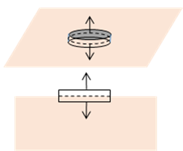
From $\overrightarrow{\nabla }\cdot \overrightarrow{B}=0,$ applying Gauss’ theorem to the usual “pillbox” infinitesimal volume enclosing the surface, the normal component of the magnetic field is continuous,

$$\left({\overrightarrow{B}}_2-{\overrightarrow{B}}_1\right)\cdot \widehat{\overrightarrow{n}}=0.$$

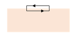
If we assume there's a free surface current ${\overrightarrow{K}}_f$ flowing along the interface, then the boundary conditions for $\overrightarrow{H}$ are (applying Stokes’ theorem for a small loop as shown)

$$\widehat{\overrightarrow{n}}\times \left({\overrightarrow{H}}_2-{\overrightarrow{H}}_1\right)={\overrightarrow{K}}_f.$$

If there are linear constitutive relations ${\overrightarrow{B}}_1={\mu }_1{\overrightarrow{H}}_1,{\overrightarrow{B}}_2={\mu }_2{\overrightarrow{H}}_2$ then

${\overrightarrow{B}}_2\times \overrightarrow{n}=\left({\mu }_2/{\mu }_1\right){\overrightarrow{B}}_1\times \overrightarrow{n},{\overrightarrow{H}}_2\cdot \overrightarrow{n}=\left({\mu }_1/{\mu }_2\right){\overrightarrow{H}}_1\cdot \overrightarrow{n},$ 

 and boundary value problems can be solved as in electrostatics.  This is true for diamagnetic and paramagnetic materials, which do behave in a linear fashion, but their response to an imposed field is weak.  For the more interesting ferromagnetic materials, the $\overrightarrow{B},\overrightarrow{H}$ curve is often complicated and history dependent.  However, there are situations in which the response is approximately linear$—$and precise answers are not always necessary.

Boundary Conditions for Vacuum/Large $\mu$ Interface

If $\mu$ is very large (as it is for ferromagnetic materials, in the thousands or more) fairly reliable conclusions can be reached with little effort, as in the following examples.

Field Lines Come Out Almost Vertically from a Strong Magnet…

If ${\mu }_1\gg {\mu }_2,$ from the boundary conditions the normal component of ${\overrightarrow{H}}_2$ is much larger than that of ${\overrightarrow{H}}_1$, whereas the tangential component (assuming no surface current) is the same for both, so in the limit of large ${\mu }_1,$ ${\overrightarrow{H}}_2$ is essentially normal to the surface, off by an angle $\sim {\mu }^{-1}$. That is, the field lines just outside a ferromagnetic material leave it almost at right angles, just like electric field lines from a conducting surface in electrostatics, with the magnet's surface corresponding to an equipotential.  This turns out to be a useful insight in designing magnets$—$and it doesn’t depend on the complications of the $\overrightarrow{B},\overrightarrow{H}$ relationship, only on ${\mu }_1\gg {\mu }_2.$

And the Reverse:

Field lines going almost, but not quite, normally into a high $\mu$ material will be bent strongly away from the normal.

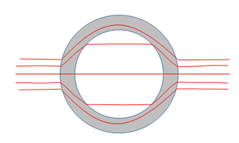
This is the basis of magnetic shielding, when it is necessary to keep out external magnetic fields.  To take a simple case, consider placing a hollow sphere of soft iron, say, in an external constant magnetic field.  

The flux line going precisely through the center is unaffected, it strikes all surfaces normally. But lines originally parallel to the central line, and close to it, are splayed outwards (the diagram here underestimates the effect).  Lines (not shown) impinging on the sphere further from the central line will all go around within the metal, so there will be a very strong field there. From the spherical symmetry plus constant external field, we know that the inside field will be constant and parallel to the outside field.  Within the metal, if we take $\mu$ constant, the strong field will be a combination of a constant field plus a dipole field, both aligned along the axis.  Jackson (section 5.12) makes this assumption, and then applying the boundary conditions gives a routine calculation to find a reduction in field ${\overrightarrow{H}}_{\text{int}}\sim {\mu }^{-1}{\overrightarrow{H}}_{\text{ext}}.$  Since the field strength in the metal varies, the actual numerical predictions are inexact, but back of the envelope arguments about how the field lines bend at boundaries confirm the order of magnitude, which is all we need.   

This kind of shielding is an active field of research: a recent publication from CERN (see its page 7) depicts two concentric high $\mu$ spheres, to achieve microtesla levels   .

Two Potentials

There was a big breakthrough in solving electrostatic problems when George Green (and independently Gauss) introduced the concept of potential, a single number at each point in space, much easier to deal with than the vector electric field.  The same general approach works in magnetostatics, but with a twist: there are two possible potentials.

1.  Magnetic Vector Potential

Since $\overrightarrow{\nabla }\cdot \overrightarrow{B}=0$, we can always write

$\overrightarrow{B}=\overrightarrow{\nabla }\times \overrightarrow{A},$

and $\overrightarrow{A}$ is called the vector potential.  But is this progress? In electrostatics, the benefit of using a potential was that scalars are a lot easier to deal with than vectors. Here we still have a vector. But the advantage here is that by working with $\overrightarrow{A},$ we are automatically ensuring that our solution satisfies Maxwell’s equation $\overrightarrow{\nabla }\cdot \overrightarrow{B}=0.$

Evidently, $\overrightarrow{A}$ is not uniquely defined: adding an arbitrary gradient term, $\overrightarrow{\nabla }\phi ,$ would not affect $\overrightarrow{B}=\overrightarrow{\nabla }\times \overrightarrow{A}.$ This makes it possible to put some constraints on $\overrightarrow{A}.$  The jargon term for this is "choosing a gauge".  For example, we can require that

$\overrightarrow{\nabla }\cdot \overrightarrow{A}=0.$ 

This is called using the Coulomb gauge, it’s important: we’ll use it a lot when discussing electromagnetic waves.  

But how do we know it’s always possible? Let's begin with a vector potential ${\overrightarrow{A}}^{\prime },$ so $\overrightarrow{B}=\overrightarrow{\nabla }\times {\overrightarrow{A}}^{\prime }$ but $\overrightarrow{\nabla }\cdot {\overrightarrow{A}}^{\prime }\ne 0.$  Now take $\overrightarrow{A}={\overrightarrow{A}}^{\prime }+\overrightarrow{\nabla }\phi ,$ where $\phi$ is the solution to the electrostatic-like equation ${\nabla }^2\phi =-\overrightarrow{\nabla }\cdot {\overrightarrow{A}}^{\prime }.$ This equation always has a solution: it’s just the electrostatic potential from a charge distribution $\overrightarrow{\nabla }\cdot \overrightarrow{A^{\prime }},$ and ${\overrightarrow{A}}^{\prime }$ is a given quantity .  Then we find $\overrightarrow{\nabla }\cdot \overrightarrow{A}=0,$ so it would have been OK to require this from the start.  (Note it still isn't quite unique:  we can add yet another term $\overrightarrow{\nabla }f$ to $\overrightarrow{A}$ provided ${\nabla }^{2}f=0.$ )

For linear media, $\overrightarrow{B}=\mu \overrightarrow{H},$ the Coulomb gauge greatly simplifies the differential equation for the potential,

$\overrightarrow{\nabla }\times \left(\overrightarrow{\nabla }\times \overrightarrow{A}\right)=\mu {\overrightarrow{j}}_f,$

becomes in the Coulomb gauge

${\nabla }^2\overrightarrow{A}=-\mu {\overrightarrow{j}}_f.$

Clearly ${\nabla }^2\overrightarrow{A}=-{\mu }_0{\overrightarrow{j}}_f$ in a vacuum (or for almost all practical purposes in a non-ferromagnetic material).  Going from ${\mu }_0$ to $\mu$ looks like a magnetic parallel to $\overrightarrow{\nabla }\cdot \overrightarrow{E}=\rho /\epsilon$  in place of $\rho /{\epsilon }_0$ in going from vacuum to a uniform dielectric$—$but it’s much more limited.  We’d need the linear $\overrightarrow{B}=\mu \overrightarrow{H}$ to be true over a range of field strengths, rarely the case, in contrast to the electrostatic $\overrightarrow{D}=\epsilon \overrightarrow{E}.$ 

2. Magnetic Scalar Potential (Regions with Zero Free Current)

In any region where the free current density is zero we have $\overrightarrow{\nabla }\times \overrightarrow{H}={\overrightarrow{j}}_{\text{free}}=0$ so we can write the field $\overrightarrow{H}$ as a gradient of a scalar magnetic potential ${\phi }_M\left(\overrightarrow{r}\right)$:

$\overrightarrow{H}\left(\overrightarrow{r}\right)=-\overrightarrow{\nabla }{\phi }_{\text{M}}\left(\overrightarrow{r}\right).$ 

We already used this for the field from a current loop. It worked everywhere in space except the actual wire (but was multivalued, since the space around the wire is not simply connected).

If we have some region in which $\mu$ is constant, then from $\overrightarrow{\nabla }\cdot \overrightarrow{B}=0$ we have

$${\nabla }^2{\phi }_{\text{M}}\left(\overrightarrow{r}\right)=0.$$

So in principle we can solve problems where there is no free current, and space is divided into regions in each of which $\mu$ is constant.

Magnetic Field from a Permanent Magnet

You’re probably thinking bar magnet, or maybe horseshoe, but the easiest to analyze with our mathematical tools is a uniformly magnetized sphere, so we’ll start there.  This is a hard ferromagnet, meaning fixed magnetization density $\overrightarrow{M}.$ There may be external magnetic fields, but the hard magnetic material is not responding to them (by definition), so $\overrightarrow{B}\ne \mu {\overrightarrow{H}}_{\text{ext}}$ here$—$in fact, we don’t need to worry about $\mu$ at all.

Scalar Potential for Magnetized Sphere

We’ll begin with a scalar magnetic potential analysis: since there are no free currents we can take $\overrightarrow{H}=-\overrightarrow{\nabla }{\phi }_M.$

Now

$\overrightarrow{\nabla }\cdot \overrightarrow{B}={\mu }_0\overrightarrow{\nabla }\cdot \left(\overrightarrow{H}+\overrightarrow{M}\right)=0,$ 

so

${\nabla }^2{\phi }_M=\overrightarrow{\nabla }\cdot \overrightarrow{M}=-{\rho }_M,$

where this ${\rho }_M$ is an effective “magnetic charge density”. 

The general solution for the scalar potential is (separating out the surface term, which could be included in the volume integral if the latter were taken over all of space):

$${\phi }_M\left(\overrightarrow{r}\right)=-\frac{1}{4\pi }{\displaystyle \underset{V}{\int }\frac{{\overrightarrow{\nabla }}^{\prime }\cdot \overrightarrow{M}\left({\overrightarrow{r}}^{\prime }\right)}{\left|\overrightarrow{r}-{\overrightarrow{r}}^{\prime }\right|}{d}^3{r}^{\prime }+}\frac{1}{4\pi }{\displaystyle \underset{S}{\int }\frac{\widehat{\overrightarrow{n}}\cdot \overrightarrow{M}\left({\overrightarrow{r}}^{\prime }\right)}{\left|\overrightarrow{r}-{\overrightarrow{r}}^{\prime }\right|}d{a}^{\prime }.}$$ 

Since we are taking the magnetization in the solid to be uniform, that first (volume) integral is zero.  

The surface term comes from a pillbox argument: $\overrightarrow{M}$ has its full value crossing one face of the pillbox, and is zero on the other. This term is often written using a surface charge density of “magnetic matter”,

$\widehat{\overrightarrow{n}}\cdot \overrightarrow{M}\left({\overrightarrow{r}}^{\prime }\right)={\sigma }_M\left({\overrightarrow{r}}^{\prime }\right)=M\cos \theta .$ 

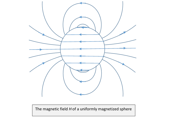
So there is positive “magnetic charge” on the right-hand side of the sphere (see diagram), negative on the left-hand side. Notice how the field lines go from positive to negative “charge”.

The argument is exactly parallel to the electrostatic analysis of a polarized dielectric sphere, which (with uniform polarization $\overrightarrow{P}$ ) has surface electric charge density $P\cos \theta ,\left(P=\rho \delta \right)$ which generates an internal electric field

$$\overrightarrow{E}=-\overrightarrow{P}/3{\epsilon }_0.$$

 Correspondingly, a sphere having uniform magnetization $\overrightarrow{M}$ generates an internal field

$$\overrightarrow{H}=-\overrightarrow{M}/3.$$

So the actual magnetic field inside the sphere

$$\overrightarrow{B}={\mu }_0\left(\overrightarrow{H}+\overrightarrow{M}\right)=\frac{2}{3}{\mu }_0\overrightarrow{M}.$$

Here’s a plot of the magnetic field $\overrightarrow{B}:$  

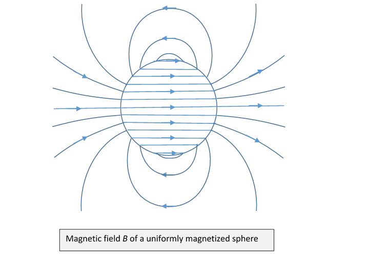
Since $\overrightarrow{\nabla }\cdot \overrightarrow{B}=0,$ field lines cannot begin or end, they loop around in this case.

Outside the sphere the field is that of a dipole of strength $V\overrightarrow{M}.$ (This exact result is only true for a sphere.)

Vector Potential for Magnetized Sphere

Taking $\overrightarrow{B}=\overrightarrow{\nabla }\times \overrightarrow{A}$, since $\overrightarrow{\nabla }\times \overrightarrow{H}={\overrightarrow{j}}_{\text{free}}=0,$ then $\overrightarrow{\nabla }\times \overrightarrow{B}={\mu }_0\overrightarrow{\nabla }\times \overrightarrow{M}={\overrightarrow{j}}_M,$ the effective current density.

In the Coulomb gauge, this leads to

${\nabla }^2\overrightarrow{A}=-{\mu }_0{\overrightarrow{j}}_M$ 

from which

$$\overrightarrow{A}\left(\overrightarrow{r}\right)=\frac{{\mu }_0}{4\pi }{\displaystyle \underset{V}{\int }\frac{{\overrightarrow{\nabla }}^{\prime }\times \overrightarrow{M}\left({\overrightarrow{r}}^{\prime }\right)}{\left|\overrightarrow{r}-{\overrightarrow{r}}^{\prime }\right|}}{d}^3{r}^{\prime }+\frac{{\mu }_0}{4\pi }{\displaystyle \underset{S}{\int }\frac{\overrightarrow{M}\left({\overrightarrow{r}}^{\prime }\right)\times \widehat{\overrightarrow{n}}}{\left|\overrightarrow{r}-{\overrightarrow{r}}^{\prime }\right|}d{a}^{\prime }}.$$ 

For a uniformly magnetized body, $\overrightarrow{\nabla }\times \overrightarrow{M}=0$ in the solid, so the only contribution to $\overrightarrow{A}$ is the second term: the effective surface current.

In an obvious notation,

$$\overrightarrow{A}\left(\overrightarrow{r}\right)=\frac{{\mu }_0}{4\pi }{\displaystyle \underset{S}{\int }\frac{{\overrightarrow{j}}_S\left({\overrightarrow{r}}^{\prime }\right)}{\left|\overrightarrow{r}-{\overrightarrow{r}}^{\prime }\right|}d{a}^{\prime }},$$ 

and the currents ${\overrightarrow{j}}_S=\overrightarrow{M}\times \overrightarrow{n}$ are along the lines of latitude (taking $\overrightarrow{M}$ as the axis)  and proportional to sin $\theta$ (here $\theta$ is the colatitude, zero at the pole).  This is exactly the current distribution of a rotating uniformly charged spherical shell!

Bar Magnet

To illustrate a bit more clearly the qualitative difference between the $\overrightarrow{B}$ field and the $\overrightarrow{H}$ field, we’ll sketch the fields for a cylindrical bar magnet having uniform magnetization $\overrightarrow{M},$ following Purcell.

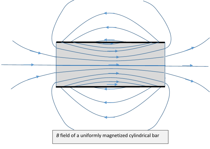
First, the $\overrightarrow{B}$ field is generated by currents $\overrightarrow{\nabla }\times \overrightarrow{M}$ which are azimuthal on the curved surface, zero on the ends, thus equivalent to a solenoid coincident with the curved surface of the bar. The field lines form closed loops with discontinuous change in derivative at the curved surface, but passing smoothly through the ends of the bar: a solenoid field.

Next, the $\overrightarrow{H}$ field. Here the two ends of the bar have uniform coverings of “magnetic matter” of opposite sign. The cylindrical curved surface plays no role, the lines cross it smoothly.

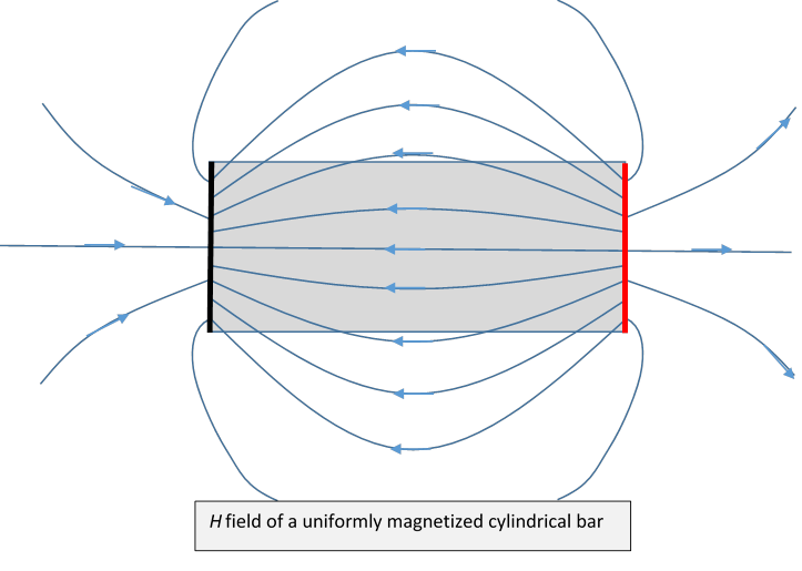
Outside the bar, the fields are identical (note: these are just sketches!), inside the bar, the fields differ by the constant magnetization. 

 Magnetized Sphere in an External Field

(Jackson 5.11) Not much useful in this section.  Two cases to be carefully distinguished: is this a hard ferromagnetic material whose magnetism is unaffected by the presence of an external field, or a soft$—$permeable$—$material, whose magnetism is caused by dipole orientation in the external field?

Hard Material: this is a rather trivial case: it doesn't respond, so we simply add the external field.

We found the magnetic field inside with no external field to be ${\overrightarrow{B}}_{\text{inside}}={\mu }_0\left(\overrightarrow{H}+\overrightarrow{M}\right)=\frac{2}{3}{\mu }_{0}M.$ 

Adding an external field ${\overrightarrow{B}}_0,$ 

${\overrightarrow{B}}_{\text{inside}}={\overrightarrow{B}}_0+\frac{2}{3}{\mu }_0\overrightarrow{M},{\mu }_0{\overrightarrow{H}}_{\text{inside}}={\overrightarrow{B}}_0-\frac{1}{3}\overrightarrow{M}.$

Soft Material: Now take it that the magnetization is caused by the external field, precisely analogous to the polarization of a dielectric sphere in an external field , so $\overrightarrow{B}=\mu \overrightarrow{H}$ inside.

This gives the magnetization in terms of the imposed field:

$\overrightarrow{M}=\frac{3}{{\mu }_0}\left(\frac{\mu -{\mu }_0}{\mu +2{\mu }_0}\right){\overrightarrow{B}}_0,$ 

only relevant for diamagnetic and paramagnetic materials, clearly not ferromagnets!

Jackson 5.12 covered earlier, 5.13 and 5.14 we skip.

previous  index  next