51 Causality and the Kramers-Krönig Relations

    Michael Fowler, UVa

(Jackson 7.10)

Causality: Polarization as a Response to a Field

The frequency dependence of  $\epsilon \left(\omega \right)$ reflects the time lag in the response of material polarization to an imposed field: recall $\overrightarrow{D}=\epsilon \overrightarrow{E}={\epsilon }_0\overrightarrow{E}+\overrightarrow{P}.$ The ${\epsilon }_0$ term indicates an instantaneous local response (really more of a change in notation than a physical transformation) but the contribution to $\overrightarrow{D}$ from the polarization $\overrightarrow{P}$ takes a finite time, because it's response of a material to a force: even electronic oscillators take time to respond fully when a driving force is switched on.

This is not so evident in frequency space, where we write

$\overrightarrow{D}\left(\overrightarrow{x},\omega \right)=\epsilon \left(\omega \right)\overrightarrow{E}\left(\overrightarrow{x},\omega \right),$ 

but that equation describes the material response to a monochromatic field, therefore one that has been oscillating forever. 

To analyze response to a field that's switched on in time, we need to go to the Fourier transforms, summing over frequencies to get the appropriate time dependence:

$\overrightarrow{D}\left(\overrightarrow{x},t\right)=\frac{1}{2\pi }{\displaystyle \underset{-\infty }{\overset{\infty }{\int }}\overrightarrow{D}\left(\overrightarrow{x},\omega \right)e^{-i\omega t}d\omega ,}\overrightarrow{D}\left(\overrightarrow{x},\omega \right)={\displaystyle \underset{-\infty }{\overset{\infty }{\int }}\overrightarrow{D}\left(\overrightarrow{x},t\right)e^{i\omega t}dt,}$ 

$\begin{array}{c}\overrightarrow{D}\left(\overrightarrow{x},t\right)=\frac{1}{2\pi }{\displaystyle \underset{-\infty }{\overset{\infty }{\int }}\overrightarrow{D}\left(\overrightarrow{x},\omega \right)e^{-i\omega t}d\omega }=\frac{1}{2\pi }{\displaystyle \underset{-\infty }{\overset{\infty }{\int }}\epsilon \left(\omega \right)\overrightarrow{E}\left(\overrightarrow{x},\omega \right)e^{-i\omega t}d\omega }\\ =\frac{1}{2\pi }{\displaystyle \underset{-\infty }{\overset{\infty }{\int }}\epsilon \left(\omega \right){\displaystyle \underset{-\infty }{\overset{t}{\int }}\overrightarrow{E}\left(\overrightarrow{x},t^{\prime }\right)e^{i\omega t^{\prime }}{e}^{-i\omega t}}d{t}^{\prime }d\omega }.\end{array}$

Notation: We use the standard physics normalization of Fourier transforms, writing $d\omega /2\pi$ and $dt.$ In this section (7.10) Jackson uses the mathematician’s convention, $d\omega /\sqrt{2\pi },dt/\sqrt{2\pi },$ even though he used the physics normalization earlier, for example in equations 6.33, 6.34.)

This is from Jackson, but we've made one slight change: this section is headed causality, the equation describes how the electric field at time $t^{\prime }$ at point $\overrightarrow{x}$ generates polarization that contributes to the field at the same point $\overrightarrow{x}$ at a later time $t.$ Think of it as a local damped oscillator at $\overrightarrow{x}$ that has been subject to a time-varying driving force $\overrightarrow{E}\left(\overrightarrow{x},t^{\prime }\right),$ and we're now finding its phase and amplitude at time $t.$ 

Obviously, this can only depend on the driving force at earlier times, so we integrate $d{t}^{\prime }$ up to $t,$ not to infinity. It's convenient to introduce the time difference variable, $t-t^{\prime }=\tau .$ This gives $d{t}^{\prime }=-d\tau ,$ but the range of integration goes from $\left(-\infty ,t\right)$ to $\left(\infty ,0\right)$ which we then switch to $\left(0,\infty \right)$ giving a second minus sign.

Finally, writing  $\epsilon \left(\omega \right)=1+{\chi }_e\left(\omega \right),$ (from lecture 29),

$\begin{array}{c}\overrightarrow{D}\left(\overrightarrow{x},t\right)=\frac{1}{2\pi }{\displaystyle \underset{-\infty }{\overset{\infty }{\int }}\epsilon \left(\omega \right){\displaystyle \underset{0}{\overset{\infty }{\int }}\overrightarrow{E}\left(\overrightarrow{x},t-\tau \right)e^{-i\omega \tau }}d\tau d\omega },\\ =\frac{{\epsilon }_0}{2\pi }{\displaystyle \underset{-\infty }{\overset{\infty }{\int }}\left(1+{\chi }_e\left(\omega \right)\right){\displaystyle \underset{0}{\overset{\infty }{\int }}\overrightarrow{E}\left(\overrightarrow{x},t-\tau \right)e^{-i\omega \tau }}d\tau d\omega }.\end{array}$.

  Actually, we should have treated this term separately from the start: it's the instant vacuum response of $\overrightarrow{D}$ to $\overrightarrow{E},$ and by (unnecessarily) incorporating it in the integral we've made things slightly awkward, the ${\displaystyle {\int }_{-\infty }^{\infty }\frac{d\omega }{2\pi }{e}^{-i\omega t}}$ integral  gives $\delta \left(\tau \right)$ and we end the integral at $\tau =0,$ we need $\tau =0_{-}$ to make sense.  Maybe this is why Jackson went to infinity, but I think doing that obscures the causal nature of the equation. 

Having dealt with the first term in $\overrightarrow{D}={\epsilon }_0\overrightarrow{E}+\overrightarrow{P},$ let's focus on the less trivial second term.

We'll define the Green's function

$\begin{array}{c}G\left(\tau \right)=\frac{1}{2\pi }{\displaystyle \underset{-\infty }{\overset{\infty }{\int }}\left[\left(\epsilon \left(\omega \right)/{\epsilon }_0\right)-1\right]}{e}^{-i\omega \tau }d\omega ,\\ =\frac{1}{2\pi }{\displaystyle \underset{-\infty }{\overset{\infty }{\int }}{\chi }_e\left(\omega \right)}{e}^{-i\omega \tau }d\omega \end{array}$ 

assuming with Jackson that the reversal of order of integrations is OK.

Note:  We’re assuming throughout that the response at $\overrightarrow{x}$ does not depend on the earlier field at some different point ${\overrightarrow{x}}^{\prime }:$ that is, we’re assuming nonlocality in time, but locality in space. This works well for dielectrics including in the visible range, but breaks down for metals if the mean free path of electrons between collisions exceeds the scale of field variation (for example, skin depth). In practice, this only occurs with very pure metals at very low (helium) temperatures, and very high frequencies (GHz). it’s called the anomalous skin effect. 

Simple Model for $G\left(\tau \right)$

To illustrate the technique, we'll assume initially that there is only one resonant frequency:

$\frac{\epsilon \left(\omega \right)}{{\epsilon }_0}-1=\frac{{\omega }_p^2}{{\omega }_0^2-{\omega }^2-i\gamma \omega },$ 

so

$G\left(\tau \right)=\frac{{\omega }_p^2}{2\pi }{\displaystyle \underset{-\infty }{\overset{\infty }{\int }}\frac{e^{-i\omega \tau }}{{\omega }_0^2-{\omega }^2-i\gamma \omega }}d\omega .$ 

(In fact, not a bad approximation in the region near that frequency.)

 We can evaluate this by contour integration.  Notice that for positive $\tau ,$ the $e^{-i\omega \tau }$ term diverges in the upper half plane, so we must complete the contour along the real axis with a large semicircle in the lower half plane.  

For negative $\tau ,$ we must complete the contour with a semicircle in the upper half plane. 

The only singularities in the integrand are the two poles at the roots of the equation ${\omega }_0^2-{\omega }^2-i\gamma \omega =0.$ 

They are poles in the lower half plane at ${\omega }_{1,2}=-\frac{1}{2}i\gamma \pm {\nu }_0,{\nu }_0^2={\omega }_0^2-\frac{1}{4}{\gamma }^2.$ 

Hence, for $\tau >0,$ 

$G\left(\tau \right)={\omega }_p^2{e}^{-\gamma \tau /2}\frac{\sin {\nu }_0\tau }{{\nu }_0}\theta \left(\tau \right),$ 

and (reassuringly!) for $\tau <0,G\left(\tau \right)=0.$ 

The analyticity of $G\left(\omega \right)$ in the upper half complex plane is equivalent to causality.

(From quantum mechanics, the width of a spectral line ( $\sim \gamma$ ) is the inverse of the lifetime of the excited state, so the Green’s function decays in a time of order the lifetime of the state, of order microseconds to nanoseconds.)

Causality and Analyticity of $\epsilon \left(\omega \right)$ 

We have established that

$\overrightarrow{D}\left(\overrightarrow{x},t\right)={\epsilon }_0\left[\overrightarrow{E}\left(\overrightarrow{x},t\right)+{\displaystyle \underset{0}{\overset{\infty }{\int }}G\left(\tau \right)\overrightarrow{E}\left(\overrightarrow{x},t-\tau \right)d\tau }\right].$ 

Now these are real values of fields at some instant in time, not frequency components that could have phase lags, so the Green's function $G\left(\tau \right)$ is real.

Recalling its definition as the Fourier transform of ${\chi }_e\left(\omega \right),$ 

$G\left(\tau \right)=\frac{1}{2\pi }{\displaystyle \underset{-\infty }{\overset{\infty }{\int }}\left[\left(\epsilon \left(\omega \right)/{\epsilon }_0\right)-1\right]}{e}^{-i\omega \tau }d\omega ,$ 

we can Fourier transform back to find,

$\frac{\epsilon \left(\omega \right)}{{\epsilon }_0}=1+{\displaystyle \underset{0}{\overset{\infty }{\int }}G\left(\tau \right)e^{i\omega \tau }d\tau }.$ 

Since $G\left(\tau \right)$ is real, it follows that

$$\frac{\epsilon \left(-\omega \right)}{{\epsilon }_0}=\frac{{\epsilon }^{\ast }\left({\omega }^{\ast }\right)}{{\epsilon }_0}.$$ 

It is apparent from the formula for $\epsilon \left(\omega \right)$ in terms of $G\left(\tau \right)$ that $\epsilon \left(\omega \right)$ is analytic in the upper half plane, and if we can assume $G\left(\tau \right)$ is finite and goes to zero at infinite time, then this is also true down to the real axis. 

(Note: This doesn't work for conductors:  recall $\epsilon \left(\omega \right)={\epsilon }_b+i\left(\sigma /\omega \right),$ there is a pole at the origin. To understand what this does to the Green's function, we must go back to $G\left(\tau \right)=\frac{1}{2\pi }{\displaystyle \underset{-\infty }{\overset{\infty }{\int }}\left[\left(\epsilon \left(\omega \right)/{\epsilon }_0\right)-1\right]}{e}^{-i\omega \tau }d\omega$.  The integrand will now include a term $i\sigma /\omega {\epsilon }_0,$ and the integral over the whole real line must include a small semicircle in the upper half plane around the origin, the formula is $1/\omega =P/\omega -i\pi \delta \left(\omega \right).$ This pole gives a time-independent contribution $\sigma /{\epsilon }_0$ to $G\left(\tau \right),$ the other terms are from oscillators with finite damping, and die away for long times.)

Kramers-Krönig Relations

Since $\epsilon \left(\omega \right)/{\epsilon }_0$ is analytic in the upper half plane, we can use Cauchy's theorem to relate the real and imaginary parts.  The real part ${\epsilon }^{\prime }\left(\omega \right)/{\epsilon }_0$ is the square of the refractive index, the imaginary part is the absorption.  Note that if a medium has a refractive index different from that of the vacuum (as all do!) then there must be nonzero absorption in some frequency range.

For any $z$ in the upper half plane, the only singularity in the integrand below is at ${\omega }^{\prime }=z,$ a simple pole, so for a contour encircling the upper half plane, 

$\frac{\epsilon \left(z\right)}{{\epsilon }_0}-1=\frac{1}{2\pi i}{\displaystyle \underset{C}{\oint }\frac{\left[\left(\epsilon \left({\omega }^{\prime }\right)/{\epsilon }_0\right)-1\right]}{{\omega }^{\prime }-z}d{\omega }^{\prime }}$ .

Since we know $\left(\epsilon \left(\omega \right)/{\epsilon }_0\right)-1\sim {\omega }^{-2}$ at infinity, we can neglect the contribution from the large semicircle, leaving

$\frac{\epsilon \left(z\right)}{{\epsilon }_0}=1+\frac{1}{2\pi i}{\displaystyle \underset{-\infty }{\overset{\infty }{\int }}\frac{\left[\epsilon \left({\omega }^{\prime }\right)/{\epsilon }_0-1\right]}{{\omega }^{\prime }-z}d{\omega }^{\prime }}$ 

We now take the point in the upper half plane to be infinitesimally above the real axis,

$\frac{\epsilon \left(\omega \right)}{{\epsilon }_0}=1+\frac{1}{2\pi i}{\displaystyle \underset{-\infty }{\overset{\infty }{\int }}\frac{\left[\epsilon \left({\omega }^{\prime }\right)/{\epsilon }_0-1\right]}{{\omega }^{\prime }-\omega -i\delta }d{\omega }^{\prime }}$ 

and now use the identity

$\frac{1}{{\omega }^{\prime }-\omega -i\delta }=\frac{P}{{\omega }^{\prime }-\omega }+i\pi \delta \left({\omega }^{\prime }-\omega \right)$ 

to find

$\begin{array}{l}{\epsilon }^{\prime }\left(\omega \right)/{\epsilon }_0=1+\frac{1}{\pi }P{\displaystyle \underset{-\infty }{\overset{\infty }{\int }}\frac{{\epsilon }^{″}\left({\omega }^{\prime }\right)/{\epsilon }_0}{{\omega }^{\prime }-\omega }}d{\omega }^{\prime },\\ {\epsilon }^{″}\left(\omega \right)/{\epsilon }_0=-\frac{1}{\pi }P{\displaystyle \underset{-\infty }{\overset{\infty }{\int }}\frac{{\epsilon }^{\prime }\left({\omega }^{\prime }\right)/{\epsilon }_0-1}{{\omega }^{\prime }-\omega }}d{\omega }^{\prime },\end{array}$

Remember now that $\epsilon \left(-\omega \right)={\epsilon }^{\ast }\left({\omega }^{\ast }\right),$ so ${\epsilon }^{\prime }\left(\omega \right)$ is even, ${\epsilon }^{″}\left(\omega \right)$ is odd$—$and we can put positive and negative frequencies together, 

$$\begin{array}{l}{\epsilon }^{\prime }\left(\omega \right)/{\epsilon }_0=1+\frac{2}{\pi }P{\displaystyle \underset{0}{\overset{\infty }{\int }}\frac{{\omega }^{\prime }{\epsilon }^{″}\left({\omega }^{\prime }\right)/{\epsilon }_0}{{{\omega }^{\prime }}^2-{\omega }^2}}d{\omega }^{\prime },\\ {\epsilon }^{″}\left(\omega \right)/{\epsilon }_0=-\frac{2\omega }{\pi }P{\displaystyle \underset{0}{\overset{\infty }{\int }}\frac{{\epsilon }^{\prime }\left({\omega }^{\prime }\right)/{\epsilon }_0-1}{{{\omega }^{\prime }}^2-{\omega }^2}}d{\omega }^{\prime }.\end{array}$$

that can be added.)

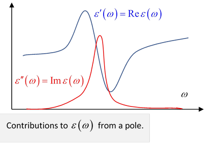
It's worth relating these equations to our model of the dielectric in terms of a set of oscillators. Think about the complex function $\epsilon \left(z\right)$ in the neighborhood of one of the poles, it's proportional to

$$\epsilon \left(z\right)\sim \frac{1}{z-z_0}=\frac{1}{\omega -\left({\nu }_0-i\frac{1}{2}\gamma \right)}.$$

How does this function vary on going along the real axis past the pole?  There is a peak in the imaginary part, its width of order $\gamma$ and its height $2/\gamma$.  The contribution from this pole to the real part of $\epsilon \left(\omega \right)$ changes sign and essentially cancels.   

Physical Significance of the Kramers-Krönig Equations

The function ${\epsilon }^{\prime }\left(\omega \right)/{\epsilon }_0$ is just the square of the refractive index $n\left(\omega \right).$ The first equation tells us that the refractive index of a material for light at a given frequency depends entirely on the rate of absorption of radiation, suitably weighted, summed over all frequencies.  The refractive index would be unity (no refraction) if the material didn't absorb at some frequency.

And, the reason we can write these equations at all is that $\epsilon \left(\omega \right)$ is analytic as a function of a complex variable in the upper half plane.

The analyticity follows directly from causality: the Fourier transform of $\epsilon \left(\omega \right),G\left(\tau \right)$ measures the response of the medium to an imposed field at a given time, and can only be nonzero at later times.

But that's true for all physical processes, in particular the response of an atom, a nucleus or an elementary particle to an ingoing wave. And any of these systems can be modeled in terms of oscillators. The scattering of one elementary particle off another is described in terms of a scattering matrix: a matrix rather than a simple function because there are multiple outcomes possible. Each possible outcome is a scattering matrix element, just a function of energy (and possible angular momentum) and these functions obey Kramers-Krönig equations. They have similar behavior to that shown above, and resonances correspond to excited states of the particle, that is, unstable heavier particles.  For particle scattering, the analogue of the refractive index is the phase shift of the wave function, so measuring these phase shifts can indicate the presence of resonances, other particles, at different energies.

Sum Rules

We’ve already met a sum rule: recall in lecture 47 we generalized the permittivity from a single oscillator

$$\frac{\epsilon \left(\omega \right)}{{\epsilon }_0}=1+\frac{N{e}^2}{{\epsilon }_{0}m\left({\omega }_0^2-{\omega }^2-i\gamma \omega \right)}$$

to a collection of similar oscillators, to find

$$\frac{\epsilon \left(\omega \right)}{{\epsilon }_0}=1+\frac{N{e}^2}{{\epsilon }_{0}m}{\displaystyle \sum _j\frac{f_j}{{\omega }_j{}^2-{\omega }^2-i{\gamma }_j\omega }}$$

where $f_j$ is the number of electrons in a molecule with parameters ${\omega }_j,{\gamma }_j,$ and now $N$ is the number of molecules in unit volume.  Generally, these oscillations are lightly damped, ${\gamma }_j$ is small, so $\epsilon \left(\omega \right)$ has a very small imaginary part except very close to one of the ${\omega }_j$ 's.

The oscillator strengths satisfy a sum rule, ${\displaystyle \sum _j{f}_j=1.}$ (Derived from the knowledge that at high frequencies $\frac{{\epsilon }_{\text{pl}}\left(\omega \right)}{{\epsilon }_0}\cong 1-\frac{{\omega }_{\text{pl}}^2}{{\omega }^2},{\omega }_{\text{pl}}^2=\frac{n_e{e}^2}{{\epsilon }_{0}m},$ all the electrons are essentially free.)

Suppose now we take the first of the Kramers-Krönig equations

$${\epsilon }^{\prime }\left(\omega \right)/{\epsilon }_0=1+\frac{2}{\pi }P{\displaystyle \underset{0}{\overset{\infty }{\int }}\frac{{\omega }^{\prime }{\epsilon }^{″}\left({\omega }^{\prime }\right)/{\epsilon }_0}{{{\omega }^{\prime }}^2-{\omega }^2}}d{\omega }^{\prime }$$

in the limit $\omega \to \infty ,$ to find ( $P$ is now irrelevant)

$$1-\frac{{\omega }_{\text{pl}}^2}{{\omega }^2}=1+\frac{2}{\pi {\omega }^2{\epsilon }_0}{\displaystyle \underset{0}{\overset{\infty }{\int }}{\omega }^{\prime }{\epsilon }^{″}\left({\omega }^{\prime }\right)}d{\omega }^{\prime },$$

or

$${\omega }_{\text{pl}}^2=+\frac{2}{\pi {\epsilon }_0}{\displaystyle \underset{0}{\overset{\infty }{\int }}{\omega }^{\prime }{\epsilon }^{″}\left({\omega }^{\prime }\right)}d{\omega }^{\prime }.$$

This means that the sum rule found for oscillators is still true for more general functions, but the reality of $G\left(\tau \right)$ means these functions have the same reality/symmetry constraints, so the complex $\epsilon \left(z\right)$ can be represented by an if necessary infinite number of oscillators$—$for example, a cut in the complex plane is equivalent within that plane to an infinite number of infinitesimal poles, etc.

Jackson presents a second sum rule, that the average value of ${\epsilon }^{\prime }\left(\omega \right)/{\epsilon }_0$ over all frequencies is unity. Looking at the expression (and the graph) for a single oscillator, it is clearly true in that case. Adding many oscillators, with strengths obeying the sum rule, it is again the case. As argued above, any $\epsilon \left(z\right)$ (with the required symmetry and reality conditions) can be approximated as a sum over oscillators, so the result follows.

Jackson 7.11: Arrival of a Signal After Propagation through a Dispersive Medium

This is a depreciated version of the treatment in the Second Edition of Jackson. Jackson evidently thinks it’s not as important as he once did, so we’ll just mention it here.  If you find it interesting, look in the Second Edition. The first point is that the signal cannot arrive faster than light in a vacuum, this follows from very general analyticity properties of the permittivity. Next comes a discussion of precursors, work done around 1914 by Sommerfeld and Brillouin. A signal having a sharp leading edge is sent into a dielectric, and subsequently detected. The first precursor (Sommerfeld) is a weak high frequency signal. This is perhaps not surprising: the required sharp initial edge needed high frequency components, and presumably they will outrun the others? The second precursor is more interesting, the Brillouin precursor. This is low frequency, and quite strong, and chirps.  A proper mathematical treatment takes a substantial amount of work, and we just don’t have time here.  However, this subject is of more than academic interest$—$googling Brillouin precursor reveals fairly extensive discussion of possible related problems in 5G communications.

previous  index  next