56  Resonant Cavities and Schumann Resonances

    Michael Fowler, UVa

Resonant Cavities

Rectangular Box

 We won't spend long on resonant cavities, because we've already covered the necessary mathematical tools in discussing waveguides.

A simple example of a cavity is a box, a section (length $d$ ) of a rectangular wave guide with the two ends blocked off with flat sheets of conductor, perpendicular to the guide walls.  So the analysis in the transverse directions is identical to that above, but in the $z$ -direction we must replace plane waves with standing waves.

The important new element is the boundary conditions at the ends: the tangential electric field and the normal magnetic field must both be zero.

TM Mode

Recall we found for the waveguide that

$E_x=\frac{i}{\mu \epsilon {\omega }^2-k^2}k\frac{\partial E_z}{\partial x},E_y=\frac{i}{\mu \epsilon {\omega }^2-k^2}k\frac{\partial E_z}{\partial y}$ 

 but the $ik$ factor came from applying $\partial /\partial z$ to a plane wave!  

For the cavity we must have a standing wave in the $z$ -direction, the wavenumber $k$ becomes $p\pi /d,$ and of course sine goes to cosine, etc.

Exercise:  Check this from the derivation in lecture 54.

For a cavity with ends $\left(0,d\right),$ to get ${\overrightarrow{E}}_t=0$ on the endplates requires a standing wave with zero derivative there,

$E_z\left(x,y,z\right)=\psi \left(x,y\right)\cos \left(\frac{p\pi z}{d}\right),$ 

so

${\overrightarrow{E}}_t=-\frac{p\pi }{d\left[\mu \epsilon {\omega }^2-{\left(p\pi /d\right)}^2\right]}\sin \left(\frac{p\pi z}{d}\right){\overrightarrow{\nabla }}_t\psi \left(x,y\right).$ 

Notice now that

${\overrightarrow{H}}_t=-\frac{i\epsilon \omega }{\mu \epsilon {\omega }^2-{\left(p\pi /d\right)}^2}\cos \left(\frac{p\pi z}{d}\right)\widehat{\overrightarrow{z}}\times {\overrightarrow{\nabla }}_t\psi \left(x,y\right),$ 

so for this standing wave, the maximum electric field values are the minimum magnetic field values.  There is a nonzero magnetic field at the ends, but it's transverse (this is a TM wave), and arises from surface currents in the end plates.

TE Mode

For the TE mode,

$H_z=\psi \left(x,y\right)\sin \left(\frac{p\pi z}{d}\right)$ 

(It has to go to zero at the two ends.)  From this,

$\begin{array}{l}{\overrightarrow{E}}_t=-\frac{i\omega \mu }{d\left[\mu \epsilon {\omega }^2-{\left(p\pi /d\right)}^2\right]}\sin \left(\frac{p\pi z}{d}\right)\widehat{\overrightarrow{z}}\times {\overrightarrow{\nabla }}_t\psi \left(x,y\right),\\ {\overrightarrow{H}}_t=-\frac{p\pi }{\mu \epsilon {\omega }^2-{\left(p\pi /d\right)}^2}\cos \left(\frac{p\pi z}{d}\right){\overrightarrow{\nabla }}_t\psi \left(x,y\right).\end{array}$ 

As before, ${\overrightarrow{E}}_t$ has to be zero at the end plates, ${\overrightarrow{H}}_t$ doesn't.

Circular Cylindrical Cavity

A right circular cylinder, inner radius $R,$ is an important cavity shape: it can be adjusted (tuned) with a piston configuration.  The math is exactly as before, except this time the 2-D wave equation has a circular boundary, and the relevant eigenfunctions of the 2-D ${\nabla }_t^2$ operator are the Bessel functions $J_m\left(x\right)$ (for a reminder, see lecture 21.)  $x_{mn}$ is the n^th zero of $J_m\left(x\right),$ so $m=0,1,2,\dots ,n=1,2,\dots$

The TM mode must have $E_z=0$ on the cylindrical walls (but not the end walls), so

$\begin{array}{c}{E}_z\left(\rho ,\varphi ,z\right)=\psi \left(\rho ,\varphi \right)\cos \left(\frac{p\pi z}{d}\right),\\ \psi \left(\rho ,\varphi \right)=E_0{J}_m\left({\gamma }_{mn}\rho \right)e^{\pm im\varphi },{\gamma }_{mn}=x_{mn}/R,J_m\left(x_{mn}\right)=0.\end{array}$ 

The resonant frequencies are given by

$${\omega }_{mnp}=\frac{1}{\sqrt{\mu \epsilon }}\sqrt{\frac{x_{mn}^2}{R^2}+\frac{p^2{\pi }^2}{d^2}}.$$

The lowest TM mode has no $z$-dependence, it's $m=0,n=1,p=0$  and is termed TM_0,1,0.

The fields for this lowest mode are:

$$E_z=E_0{J}_0\left(\frac{2.405\rho }{R}\right)e^{-i\omega t},H_{\varphi }=-i\sqrt{\frac{\epsilon }{\mu }}{E}_0{J}_1\left(\frac{2.405\rho }{R}\right)e^{-i\omega t}.$$

Exercise:  Sketch how these fields change during one cycle.

For the TE modes, we have the same 2-D differential equation as above, but now the boundary condition for $B_z$ is $\partial B_z/\partial n=0,$ meaning $\partial \psi /\partial \rho =0,$ so the Bessel function must have zero slope at the boundary.   This means we must choose different scaling factors ${\gamma }_{mn}={x^{\prime }}_{mn}/R,$ where ${J^{\prime }}_m\left(x_{mn}\right)=0.$   (These zero derivative points are sometimes labeled $y_{mn}$.)  For the circular cylindrical case, then, TE and TM modes cannot have the same eigenvalue.

Power Losses in a Cavity, Q Value

The $Q$ value is just the power dissipation rate: the stored energy in the cavity, if unfed, decays exponentially:

$\frac{dU}{dt}=-\frac{{\omega }_0}{Q}U,U\left(t\right)=U_0{e}^{-{\omega }_{0}t/Q}.$ 

This defines $Q.$  The energy loss mechanism is precisely the same as we've already discussed for the waveguide, and $Q$ is effectively the ratio of the internal volume to the volume surface area $\times \delta ,$ with some geometric shape factor (usually of order one), and the appropriate correction for the case of dielectric filling. Typical $Q$ values are in the hundreds, but provided $Q\ne \infty ,$ the oscillation is actually a resonance with width $\sim {\omega }_0/Q.$  

Jackson gives a full account of the details, we’re not going to go through them here.

Schumann Resonances

Here We Are

In fact, we’re living in a resonant cavity! It’s not a bad first approximation to take the surface of the Earth to be a spherical conductor, and the ionosphere to be a concentric spherical conductor, the atmosphere between them is the dielectric filling. Charge could be exchanged between the spheres in electrical storms, and the first estimate of resonant frequencies was made in 1952 by Winfried Schumann who predicted a frequency range 3Hz to 60 Hz.  (Trivia footnote: he was a German scientist brought to the US at the end of the war by secret Operation Paperclip,  some years later he returned to Munich.)

A Simple Model

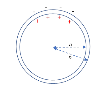
Suppose that at some moment a charge imbalance has somehow been generated as shown in the figure: excess positive charge on the Earth’s surface in an upper part of the northern hemisphere, corresponding negative charge in the ionosphere.  Let’s take it azimuthally symmetric ( $\varphi$-independent). What will happen? The charges shown (positive and negative) will flow southwards, equally at all longitudes. The currents will generate magnetic fields in the $\phi$ direction in the atmosphere, these build up then help keep the current flowing until the charge distribution is like the original one, but upside down, now centered at the south pole. Then repeat in reverse, etc.  Of course, there will be damping$—$a pretty low $Q$ value.  An order of magnitude for the oscillation frequency is given by the time it takes light to go around the Earth, of order 0.15 seconds.  Higher frequency modes could have latitudinal bands of alternating positive and negative charge, still $\varphi$-independent.

Exercise:  The energy flows in the fields! Sketch the electric and magnetic fields, and the Poynting vector, at some nontrivial time in the cycle.

Finding the Eigenfrequencies

Our picture suggests a radial electric field, that would be a TM mode, and this would certainly be the case for the lowest frequencies, otherwise (for TE) the radial component would have a wavelength of order the height of the ionosphere, $h=b-a,$ frequency $\sim c/h,$ much higher than TM modes $\sim c/a.$ So for the low frequency modes there can be no radial magnetic field, and $\overrightarrow{\nabla }\cdot \overrightarrow{B}=0$ means that the only nonzero magnetic field component is $B_{\varphi }.$ Also $E_{\varphi }=0$ from Faraday’s law. 

Following Jackson, for time dependence $e^{-i\omega t},$ the two Maxwell curl equations give

$$\frac{{\omega }^2}{c^2}\overrightarrow{B}=\overrightarrow{\nabla }\times \overrightarrow{\nabla }\times \overrightarrow{B}.$$

(You might be tempted to write curl curl = grad div $–$ del squared, but that is Cartesian. Here you need to look up curl in spherical coordinates, and use it twice$—$it comes out a little different.)

Now (from Wikipedia),  $\overrightarrow{\nabla }\times \left(0,0,B_{\varphi }\right)=\frac{1}{r\sin \theta }\frac{\partial }{\partial \theta }\left(B_{\varphi }\sin \theta \right)\widehat{\overrightarrow{r}}-\frac{1}{r}\frac{\partial }{\partial r}\left(r{B}_{\varphi }\right)\widehat{\overrightarrow{\theta }}$,

and

$$\overrightarrow{\nabla }\times \overrightarrow{\nabla }\times \left(0,0,B_{\varphi }\right)=\left(0,0,-\frac{1}{r}\frac{{\partial }^2}{\partial r^2}\left(r{B}_{\varphi }\right)-\frac{1}{r}\frac{\partial }{\partial \theta }\frac{1}{\sin \theta }\frac{\partial }{\partial \theta }\left(B_{\varphi }\sin \theta \right)\right).$$

Putting this in the equation, and multiplying throughout by $r,$ the $\varphi$ component is

$$\frac{{\omega }^2}{c^2}\left(r{B}_{\varphi }\right)+\frac{{\partial }^2}{\partial r^2}\left(r{B}_{\varphi }\right)+\frac{1}{r^2}\frac{\partial }{\partial \theta }\left[\frac{1}{\sin \theta }\frac{\partial }{\partial \theta }\left(r{B}_{\varphi }\sin \theta \right)\right]=0.$$

Following Jackson, the angular part can be written

$$\frac{\partial }{\partial \theta }\left[\frac{1}{\sin \theta }\frac{\partial }{\partial \theta }\left(r{B}_{\varphi }\sin \theta \right)\right]=\frac{1}{\sin \theta }\frac{\partial }{\partial \theta }\left[\sin \theta \frac{\partial }{\partial \theta }\left(r{B}_{\varphi }\right)\right]-\frac{r{B}_{\varphi }}{{\sin }^2\theta }.$$

Noticing now that this is the angular part of the Laplacian as given at the beginning of lecture 18, for $m=1,$ (so ${\partial }^2\phi /\partial {\varphi }^2=-\phi$ ) hence we write

$$B_{\varphi }\left(r,\theta \right)=\frac{u_l\left(r\right)}{r}{P}_l^1\left(\cos \theta \right)$$

to get

$$\frac{d^2{u}_l\left(r\right)}{d{r}^2}+\left[\frac{{\omega }^2}{c^2}-\frac{l\left(l+1\right)}{r^2}\right]u_l\left(r\right)=0.$$

The field component $E_{\theta }=-\frac{i{c}^2}{\omega r}\frac{\partial }{\partial r}\left(r{B}_{\varphi }\right)=-\frac{i{c}^2}{\omega r}\frac{\partial u_l\left(r\right)}{\partial r}{P}_l^1\left(\cos \theta \right)$ must vanish at the boundaries, meaning that $u_l\left(r\right)$ has oscillations with wavelength of order the height of the atmosphere, $h.$ These will be relatively high frequency, so the only option is $E_{\theta }=0,$ meaning  $u_l\left(r\right)$ close to constant, and eigenvalues (in this approximation)

$${\omega }_l\cong \sqrt{l\left(l+1\right)}\frac{c}{a}.$$

In fact, the measured values of the first seven resonances are approximately $5.8\sqrt{l\left(l+1\right)}\text{ Hz},$ about 20% less than this naïve prediction, surprisingly good.

Exercise: find approximate values for the “skin depth” in the ocean and in the ionosphere.

previous  index  next